A Comprehensive Guide to Bulk RNA-seq Analysis: Mastering DESeq2 and edgeR for Robust Differential Expression
This article provides a definitive guide for researchers and scientists performing differential expression analysis with DESeq2 and edgeR.
A Comprehensive Guide to Bulk RNA-seq Analysis: Mastering DESeq2 and edgeR for Robust Differential Expression
Abstract
This article provides a definitive guide for researchers and scientists performing differential expression analysis with DESeq2 and edgeR. It covers the foundational principles of bulk RNA-seq, including count data properties and the negative binomial distribution used by both tools. The guide offers detailed, step-by-step methodological workflows from data import to result interpretation, alongside practical troubleshooting advice for common issues. Furthermore, it presents a comparative analysis of DESeq2 and edgeR, evaluating their performance across different sample sizes and data types to help users select the optimal tool. The content is designed to empower professionals in genomics and drug development to conduct statistically sound and biologically relevant transcriptomic studies.
Laying the Groundwork: Core Concepts and Data Preparation for Bulk RNA-seq
RNA sequencing (RNA-seq) has revolutionized transcriptomics by enabling genome-wide quantification of RNA abundance with high resolution and accuracy [1]. A fundamental characteristic of RNA-seq data is its count-based nature, where expression values represent discrete, non-negative integers corresponding to the number of sequencing reads mapped to each gene [2]. These counts are inherently noisy and exhibit substantial variability, necessitating specialized statistical models that can properly account for their unique distributional properties [2]. The core challenge in analyzing this data stems from its high-dimensional structure—typically tens of thousands of genes measured across a limited number of samples—combined with multiple sources of biological and technical variation [1] [3].
The selection of an appropriate statistical distribution for modeling RNA-seq counts is not merely a technical formality but a critical determinant of analytical accuracy. Improper models can lead to inflated false discovery rates, reduced power to detect true differential expression, and ultimately, unreliable biological conclusions [4] [5]. Among the various distributions considered for count data, the negative binomial distribution has emerged as the cornerstone for differential expression analysis in bulk RNA-seq workflows, particularly in widely adopted tools such as DESeq2 and edgeR [2] [6]. This preference stems primarily from its ability to handle overdispersion—a phenomenon where the variance in fragment counts exceeds the mean—which is routinely observed in RNA-seq datasets due to biological variability and technical artifacts [2] [4].
The Limitation of Traditional Distributions for RNA-seq Data
Poisson Distribution
The Poisson distribution represents the simplest model for count data, describing the probability of a number of independent events occurring in a fixed interval of time or space [2]. It is characterized by a single parameter (λ) where the variance equals the mean (σ² = μ). This property makes it suitable for modeling rare events with low counts, such as manufacturing failures or radioactive decay [2]. However, this fundamental assumption becomes problematic for RNA-seq data because genes with identical mean expression levels frequently exhibit different variances [2]. In reality, the variance of gene counts typically exceeds the mean, a discrepancy that becomes more pronounced with increasing biological variability between samples. Consequently, the Poisson distribution tends to underestimate variability in RNA-seq data, leading to artificially narrow confidence intervals and inflated type I errors in differential expression testing [4].
Binomial Distribution
The binomial distribution models the probability of achieving a specific number of "successes" in a fixed number of independent trials, each with the same probability of success [2]. For example, it can calculate the probability of obtaining four heads after five coin tosses. This distribution is inherently limited for RNA-seq applications because it presupposes a fixed upper bound (the number of trials) and a binary outcome structure [2]. RNA-seq data, in contrast, lacks a theoretical maximum count value—sequencing depth can vary substantially between experiments—and involves quantifying expression levels across hundreds to thousands of genes with complex, continuous-like expression patterns rather than simple binary outcomes [2].
The Overdispersion Problem in RNA-seq Data
Overdispersion represents a fundamental characteristic of RNA-seq count data where the observed variance systematically exceeds what would be expected under simpler parametric models like the Poisson distribution [4]. This phenomenon arises from multiple sources, including biological variability (genetic differences, physiological states, environmental responses), technical artifacts (library preparation biases, sequencing depth variations, batch effects), and measurement errors [2] [1]. The consequences of unaccounted overdispersion are severe: statistical tests lose calibration, p-values become artificially significant, and false discovery rates increase substantially [4] [5]. This problem is particularly acute in studies with small sample sizes, where accurately estimating variability from limited data is challenging [4].
Table 1: Comparison of Statistical Distributions for RNA-seq Count Data
| Distribution | Key Characteristics | Variance Structure | Suitability for RNA-seq | Major Limitations |
|---|---|---|---|---|
| Poisson | Models rare, independent events | Variance = Mean | Poor | Underestimates true variability; fails to handle overdispersion |
| Binomial | Models fixed number of trials with binary outcomes | Variance = np(1-p) | Very Poor | Requires fixed upper limit; inappropriate for unbounded counts |
| Negative Binomial | Extension of Poisson with dispersion parameter | Variance = μ + αμ² | Excellent | Specifically designed to handle overdispersion in count data |
The Negative Binomial Distribution: Theoretical Foundation
Mathematical Formulation
The negative binomial distribution can be conceptually understood as a Poisson-gamma mixture model, where the Poisson parameter (λ) is itself a random variable following a gamma distribution [2]. This hierarchical structure provides the mathematical flexibility to accommodate extra-Poisson variation. The probability mass function for the negative binomial distribution is given by:
[ P(Y=k) = \frac{\Gamma(k+\frac{1}{\alpha})}{\Gamma(k+1)\Gamma(\frac{1}{\alpha})} \left(\frac{1}{1+\alpha\mu}\right)^{\frac{1}{\alpha}} \left(\frac{\alpha\mu}{1+\alpha\mu}\right)^k ]
where μ represents the mean of the distribution, and α ≥ 0 denotes the dispersion parameter that controls the extent of overdispersion relative to the Poisson distribution [2] [5]. The variance of the negative binomial distribution is given by Var(Y) = μ + αμ², explicitly modeling the relationship where variance increases as a quadratic function of the mean [5]. As α approaches zero, the negative binomial converges to the Poisson distribution, while larger values of α indicate greater overdispersion [2].
The Dispersion Parameter
The dispersion parameter (α) sits at the core of the negative binomial model's ability to handle RNA-seq data complexity. This parameter quantifies the extra-Poisson variation present in the counts and directly influences both the width of confidence intervals and the power of statistical tests [2] [5]. In practice, the dispersion parameter is not treated as fixed but is estimated from the data itself using empirical Bayes methods that share information across genes [6] [5]. This shrinkage approach stabilizes estimates, particularly for genes with low counts or few replicates, by borrowing strength from the overall distribution of dispersions across all genes [6] [5]. The relationship between mean expression and dispersion typically follows a predictable trend, which differential expression tools exploit to improve estimation accuracy [6].
Practical Implementation in Differential Expression Analysis
DESeq2 and edgeR: Negative Binomial-Based Workflows
DESeq2 and edgeR, the two most widely used tools for bulk RNA-seq differential expression analysis, both employ the negative binomial distribution as their statistical foundation but implement distinct approaches to parameter estimation and hypothesis testing [6]. DESeq2 utilizes a median-of-ratios normalization method to correct for differences in sequencing depth and library composition, followed by dispersion estimation using empirical Bayes shrinkage [1] [6]. The model then fits negative binomial generalized linear models (GLMs) and tests for differential expression using Wald tests or likelihood ratio tests [6] [5]. edgeR, conversely, typically applies the TMM (Trimmed Mean of M-values) normalization and offers multiple approaches for dispersion estimation, including the ability to model a common dispersion across all genes, trended dispersion based on mean expression relationships, or gene-specific dispersions [6] [5]. For hypothesis testing, edgeR provides both likelihood ratio tests and quasi-likelihood F-tests, with the latter generally offering more robust error control, particularly for studies with small sample sizes [6].
Addressing Specialized Analytical Challenges
Recent methodological developments have extended the negative binomial framework to address more complex analytical scenarios. The NBAMSeq package implements a negative binomial additive model that can capture nonlinear relationships between covariates and gene expression, which may be missed by standard linear models [5]. This flexibility is particularly valuable when analyzing the effect of continuous covariates such as age, disease severity scores, or time, where the assumption of linearity may not hold [5]. Similarly, the DEHOGT (Differentially Expressed Heterogeneous Overdispersion Genes Testing) method addresses scenarios where overdispersion patterns vary substantially between experimental conditions, improving detection power particularly in studies with limited replicates [4].
Table 2: Comparison of Negative Binomial-Based Differential Expression Tools
| Tool | Normalization Approach | Dispersion Estimation | Testing Methodology | Special Features |
|---|---|---|---|---|
| DESeq2 | Median-of-ratios | Empirical Bayes shrinkage | Wald test or LRT | Automatic outlier detection, independent filtering, strong FDR control |
| edgeR | TMM (Trimmed Mean of M-values) | Common, trended, or tagwise | Likelihood ratio test or Quasi-likelihood F-test | Efficient with small samples, multiple testing strategies |
| NBAMSeq | Median-of-ratios (DESeq2-style) | Bayesian shrinkage | Generalized additive model tests | Captures nonlinear effects, smooth functions of covariates |
| DEHOGT | Custom normalization | Heterogeneous across conditions | Likelihood-based | Handles condition-specific overdispersion, improved power for small n |
Experimental Protocols for Differential Expression Analysis
Sample Preparation and Sequencing
Proper experimental design is paramount for generating reliable RNA-seq data. Researchers should include a minimum of three biological replicates per condition, though more may be required when biological variability is high [1]. Biological replicates represent genetically distinct individuals subjected to the same experimental condition, essential for capturing population-level variability, as opposed to technical replicates which involve repeated measurements of the same biological sample [7]. For standard differential expression analyses, sequencing depths of 20-30 million reads per sample are generally sufficient, though this may increase for studies focusing on low-abundance transcripts or for detecting subtle expression changes [1]. Prior to library preparation, RNA quality should be rigorously assessed using appropriate metrics (e.g., RIN > 8), and consistent library preparation protocols should be maintained across all samples to minimize technical batch effects [1] [3].
Computational Workflow
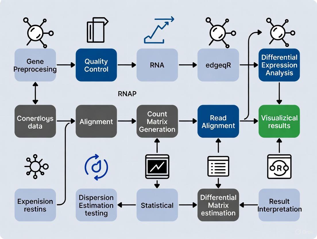
A standardized computational workflow for negative binomial-based differential expression analysis typically includes the following stages:
Quality Control and Trimming: Assess raw sequence quality using FastQC or multiQC, then remove adapter sequences and low-quality bases using tools such as fastp or Trim Galore [1] [3]. This critical first step eliminates technical artifacts that could interfere with accurate alignment and quantification.
Read Alignment and Quantification: Map cleaned reads to a reference genome or transcriptome using aligners like STAR or HISAT2, or employ alignment-free quantification with Salmon or Kallisto [8] [1] [3]. These tools incorporate statistical models to estimate transcript abundances, with Salmon being particularly noted for its accuracy and speed [8] [1].
Count Matrix Import and Preparation: Import quantification results into R/Bioconductor using specialized packages like tximeta (for Salmon output) or tximport, which automatically handle transcript-to-gene summarization and generate appropriate offset matrices to account for differential isoform usage [8].
Exploratory Data Analysis: Perform principal component analysis (PCA) and sample clustering to identify potential batch effects, outliers, or unexpected sample relationships [8] [9]. This qualitative assessment helps validate experimental integrity before formal statistical testing.
Differential Expression with Negative Binomial Models: Implement either DESeq2 or edgeR following their respective workflows, including appropriate normalization, dispersion estimation, and statistical testing [8] [6] [9]. For complex experimental designs with multiple factors, ensure the design matrix properly encodes all relevant biological conditions and technical covariates.
Results Interpretation and Visualization: Generate diagnostic plots such as MA-plots (log-fold change versus mean expression) and volcano plots to visualize differential expression results, and perform functional enrichment analysis to extract biological insights from significant gene lists [7] [9].
Figure 1: Standard RNA-seq Differential Expression Workflow
Wet-Laboratory Reagents
- RNA Extraction Kits (e.g., TRIzol, column-based kits): Maintain RNA integrity and prevent degradation during sample preparation, crucial for accurate quantification of in vivo expression levels.
- Poly-A Selection or Ribodepletion Kits: Enrich for messenger RNA by targeting polyadenylated transcripts or removing ribosomal RNA, respectively, ensuring efficient sequencing of informative transcripts.
- Reverse Transcriptase and RNA Library Prep Kits: Convert RNA to complementary DNA (cDNA) and add sequencing adapters with unique molecular identifiers to control for amplification biases.
- Quantification and Quality Control Tools (e.g., Bioanalyzer, Qubit): Precisely measure RNA concentration and integrity before library preparation, with minimum quality thresholds (RIN > 8) recommended for reliable results.
- Sequenceing Reagents and Platforms (e.g., Illumina NovaSeq, NextSeq): Generate high-throughput digital readouts of transcript abundance, with appropriate sequencing depth (20-40 million reads/sample) for the experimental design.
Computational Tools and Environments
- R and Bioconductor: Open-source statistical computing environment providing specialized packages (DESeq2, edgeR, limma) for negative binomial-based differential expression analysis [8] [6] [9].
- Python Ecosystems (InMoose, pydeseq2): Python implementations of established R tools, offering similar functionality with nearly identical results for enhanced interoperability between bioinformatics pipelines [10].
- Quality Control Pipelines (FastQC, multiQC, fastp): Assess sequence quality, adapter contamination, and other technical metrics to ensure data quality before formal analysis [1] [3].
- Alignment and Quantification Software (STAR, HISAT2, Salmon, Kallisto): Map reads to reference genomes or directly estimate transcript abundances using alignment-free methods [8] [1] [3].
- High-Performance Computing Resources: Computational clusters or cloud computing platforms capable of handling memory-intensive processing of large RNA-seq datasets, particularly for alignment and quantification steps.
Table 3: Normalization Methods for RNA-seq Count Data
| Method | Sequencing Depth Correction | Gene Length Correction | Library Composition Correction | Suitable for DE Analysis |
|---|---|---|---|---|
| CPM | Yes | No | No | No |
| RPKM/FPKM | Yes | Yes | No | No |
| TPM | Yes | Yes | Partial | No |
| Median-of-ratios (DESeq2) | Yes | No | Yes | Yes |
| TMM (edgeR) | Yes | No | Yes | Yes |
Advanced Considerations and Future Directions
As RNA-seq methodologies continue to evolve, statistical approaches must adapt to address emerging challenges. For studies incorporating multiple continuous covariates or time-series designs, extensions of the negative binomial model such as NBAMSeq offer enhanced flexibility to capture non-linear expression responses [5]. The development of methods like DEHOGT, which specifically addresses heterogeneous overdispersion across experimental conditions, demonstrates ongoing refinements to improve detection power, particularly for studies with limited sample sizes [4]. The recent emergence of cross-platform implementations such as InMoose, which provides Python equivalents of established R tools, reflects growing emphasis on interoperability and reproducibility across computational environments [10].
Future methodological developments will likely focus on integrating negative binomial models with single-cell RNA-seq analytical frameworks, addressing the even more pronounced overdispersion and zero-inflation characteristics of single-cell data. Similarly, multi-omics integration approaches that combine RNA-seq with other data types (e.g., epigenomics, proteomics) will require further extension of these foundational statistical models. Throughout these developments, the negative binomial distribution will remain central to RNA-seq analysis, providing a robust mathematical foundation for extracting meaningful biological insights from count-based sequencing data while properly accounting for their complex variability structure.
Figure 2: Statistical Distribution Comparison for RNA-seq Data
In bulk RNA-seq data analysis, normalization is a critical preprocessing step to account for technical variations, enabling meaningful biological comparisons between samples. The core challenge stems from the fact that the total number of sequenced reads (library size) can vary substantially between samples, and the RNA composition of samples may differ significantly due to biological conditions [11]. Without proper normalization, these technical artifacts can lead to false conclusions in differential expression analysis. Among the various normalization methods developed, the Median Ratio Normalization (RLE) used in DESeq2 and the Trimmed Mean of M-values (TMM) implemented in edgeR have emerged as two of the most widely adopted and robust scaling normalization methods [12] [13]. Both methods operate under the core principle that most genes are not differentially expressed across conditions, and they aim to estimate sample-specific scaling factors that minimize these technical biases. Despite their similar philosophical foundations, their statistical approaches and implementation details differ in ways that can impact analytical outcomes in specific experimental contexts.
Theoretical Foundations and Algorithmic Workflows
DESeq2's Median Ratio Normalization (RLE)
The Median Ratio Normalization method, also referred to as Relative Log Expression (RLE) normalization, is based on the fundamental assumption that the majority of genes in a dataset are not differentially expressed [11]. This method constructs a pseudo-reference sample against which all individual samples are compared. The step-by-step mathematical procedure is as follows:
Step 1: Pseudo-Reference Sample Creation - For each gene across all samples, calculate the geometric mean. This creates a virtual reference sample that represents the typical expression profile. The geometric mean for gene g is calculated as:
Geometric Mean_g = (∏_{k=1}^{n} X_{g,k})^{1/n}
where X_{g,k} represents the count for gene g in sample k, and n is the total number of samples [11].
Step 2: Ratio Calculation - For each gene in each sample, compute the ratio of its count to the corresponding pseudo-reference value:
Ratio_{g,k} = X_{g,k} / Geometric Mean_g
Step 3: Size Factor Determination - For each sample, the size factor (normalization factor) is calculated as the median of all gene ratios for that sample:
Size Factor_k = median(Ratio_{g,k})
This median-based approach makes the method robust to outliers, including highly differentially expressed genes [11].
The underlying statistical framework of DESeq2 models raw counts using a negative binomial distribution and incorporates these size factors into its generalized linear model for differential expression testing [6].
edgeR's Trimmed Mean of M-values (TMM)
The TMM normalization method also operates under the assumption that most genes are not differentially expressed, but implements a different strategy based on pairwise sample comparisons [14]. The algorithm proceeds as follows:
Step 1: Reference Sample Selection - Typically, the sample whose upper quartile of gene counts is closest to the average upper quartile across all samples is chosen as the reference, though users can specify an alternative reference [15].
Step 2: M-value and A-value Calculation - For each gene g when comparing sample k to the reference sample r, compute:
M_g = log₂((X_g/k / N_k) / (X_g/r / N_r))
A_g = ½ · log₂((X_g/k / N_k) · (X_g/r / N_r))
where X_g/k and X_g/r are counts for gene g in the test and reference samples, and N_k and N_r are the total library sizes for the respective samples [14].
Step 3: Data Trimming and Weighting - Trim the data by removing genes with extreme M-values (default: 30% from top and bottom) and genes with extreme A-values (default: 5% from each end). This trimming eliminates genes that are potentially differentially expressed or have very low expression, which could disproportionately influence the normalization [14].
Step 4: Normalization Factor Calculation - Compute the weighted mean of the remaining M-values, where weights are derived from inverse approximate variances, to obtain the log normalization factor. The final TMM scaling factor is the exponential of this value [15] [14].
edgeR incorporates these normalization factors into its statistical framework based on negative binomial generalized linear models, either as offsets or by adjusting the effective library sizes [6] [15].
Table 1: Core Algorithmic Differences Between RLE and TMM Methods
| Aspect | DESeq2's RLE (Median Ratio) | edgeR's TMM (Trimmed Mean of M-values) |
|---|---|---|
| Reference | Geometric mean across all samples (pseudo-reference) | One actual sample as reference |
| Core Calculation | Median of ratios to pseudo-reference | Weighted trimmed mean of log ratios |
| Data Trimming | Implicit via median robustness | Explicit trimming of extreme M and A values |
| Weighting Scheme | No explicit weighting | Inverse variance weighting |
| Handling of Zero Counts | Problematic for geometric mean | Genes with zero counts in either sample are excluded |
Comparative Analysis of Normalization Performance
Theoretical and Practical Comparisons
Research has demonstrated that while RLE and TMM share similar conceptual foundations, they can yield different results in practice depending on the data characteristics. A comparative study on tomato fruit set RNA-seq data showed that while RLE and MRN (a variant similar to RLE) normalization factors exhibited positive correlation with library size, TMM factors showed no significant correlation with library size [12] [13]. This fundamental difference in behavior stems from their distinct algorithmic approaches to estimating scaling factors.
In terms of performance under different experimental conditions, both methods generally perform well when the assumption of non-DE for most genes holds true. However, studies have indicated that TMM may have advantages in specific scenarios. In a hypothetical situation where case samples have half the number of expressed transcripts compared to controls (but identical sequencing depth), TMM normalization successfully corrected for this composition bias, while library size scaling alone failed dramatically [15]. The TMM method's explicit trimming of extreme values makes it particularly robust to situations where a substantial proportion of genes are differentially expressed or when there are extreme outliers [14].
Impact on Differential Expression Analysis
The choice of normalization method can significantly impact downstream differential expression results. While both methods are widely adopted and generally produce concordant results for clear differential expression patterns, discrepancies can emerge for genes with moderate fold changes or in datasets with complex expression landscapes [6]. Benchmarking studies have shown that the agreement between DEGs identified by DESeq2 and edgeR is generally high, though not perfect, with the level of concordance dependent on factors such as sample size, effect size, and data quality [6] [3].
Table 2: Performance Characteristics Under Different Experimental Conditions
| Experimental Condition | RLE (DESeq2) Performance | TMM (edgeR) Performance |
|---|---|---|
| Simple two-condition design | Excellent | Excellent |
| Large proportion of DE genes | Robust but may be influenced if majority are DE | Highly robust due to explicit trimming |
| Presence of extreme outliers | Moderately robust (median-based) | Highly robust (explicit trimming) |
| Data with high zero counts | May be problematic for geometric mean | TMMwsp variant handles zeros effectively |
| Complex multi-factor designs | Excellent (integrates with GLM) | Excellent (integrates with GLM) |
| Very small sample sizes (n < 5) | Good performance | Good performance, efficient with small samples |
Practical Implementation Protocols
DESeq2 RLE Normalization Protocol
Materials and Reagents:
- Raw count matrix (genes × samples)
- R statistical environment (version 4.0 or higher)
- DESeq2 package (version 1.30.0 or higher)
- Sample metadata table with experimental design
Experimental Procedure:
- Data Preparation: Load raw count data into R, ensuring that row names correspond to gene identifiers and column names to sample identifiers. Prepare a metadata data.frame describing the experimental design.
DESeqDataSet Creation:
Normalization Execution:
Size Factor Extraction:
Troubleshooting Tips:
- If many genes have zero counts across all samples, consider pre-filtering to improve geometric mean calculation.
- If convergence issues arise during subsequent differential expression analysis, examine size factors for extreme values that might indicate sample quality issues.
edgeR TMM Normalization Protocol
Materials and Reagents:
- Raw count matrix (genes × samples)
- R statistical environment (version 4.0 or higher)
- edgeR package (version 3.32.0 or higher)
- Sample metadata table with experimental design
Experimental Procedure:
- Data Preparation: Load raw count data as described for DESeq2 protocol.
DGEList Object Creation:
Normalization Execution:
Normalized Data Access:
Troubleshooting Tips:
- For data with high proportions of zeros, consider using method = "TMMwsp" (TMM with singleton pairing) for improved stability.
- Examine the plotMDS(dge) output to identify potential sample outliers that might unduly influence the TMM calculation.
Visualization of Normalization Workflows
DESeq2 Median Ratio Normalization (RLE) Workflow
Diagram 1: DESeq2 RLE normalization creates a pseudo-reference sample from geometric means, then calculates size factors as the median of each sample's gene ratios to this reference.
edgeR TMM Normalization Workflow
Diagram 2: edgeR TMM normalization selects a reference sample, calculates log ratios, trims extreme values, then computes weighted means to determine normalization factors.
Table 3: Key Research Reagent Solutions for RNA-Seq Normalization Studies
| Resource | Type | Function in Normalization | Example/Source |
|---|---|---|---|
| Reference RNA Samples | Biological Standard | Benchmarking normalization performance | External RNA Controls Consortium (ERCC) spikes |
| RNA Extraction Kits | Laboratory Reagent | Ensure high-quality input material | Qiagen RNeasy, TRIzol reagent |
| Library Prep Kits | Laboratory Reagent | Generate sequencing libraries | Illumina TruSeq Stranded mRNA |
| Alignment Software | Computational Tool | Generate raw count data | STAR, HISAT2, Salmon |
| Statistical Environment | Computational Platform | Execute normalization algorithms | R Statistical Environment |
| Analysis Packages | Computational Resource | Implement normalization methods | DESeq2, edgeR, limma |
| Quality Control Tools | Computational Resource | Assess normalization effectiveness | FastQC, MultiQC, ggplot2 |
Application-Specific Recommendations
The choice between DESeq2's RLE and edgeR's TMM normalization should be guided by specific experimental considerations and data characteristics. Based on comparative studies and methodological evaluations, we recommend:
For standard experimental designs with balanced conditions and no extreme global expression shifts, both methods perform excellently and will yield highly concordant results [12] [16]. The choice can be based on researcher familiarity with the respective packages for downstream analysis.
For datasets with suspected asymmetric differential expression or when a substantial proportion of genes are expected to be DE, TMM may have advantages due to its explicit trimming of extreme values, making it more robust to violations of the "most genes not DE" assumption [14].
For complex multi-factor experiments where integration with sophisticated generalized linear models is required, both methods integrate well with their respective package's modeling frameworks, and the choice may depend on which package's complete analytical workflow better suits the research question [6].
For data with unusual characteristics (extreme composition biases, very small sample sizes, or high proportions of zeros), we recommend running both normalization methods and comparing the resulting lists of differentially expressed genes. Substantial discrepancies should be investigated carefully, potentially using additional validation methods [17] [3].
DESeq2's Median Ratio Normalization and edgeR's TMM represent two sophisticated, robust, and theoretically grounded approaches to RNA-seq count normalization. While both operate under the core principle that most genes are not differentially expressed, their mathematical implementations differ significantly—RLE using a median-based approach with a pseudo-reference, and TMM employing a trimmed mean framework with an actual reference sample. Despite these differences, extensive benchmarking has demonstrated that both methods perform well across a wide range of realistic experimental scenarios, with subtle advantages emerging for each method in specific contexts. Researchers should understand the underlying assumptions of each method and select the approach most appropriate for their experimental design, while recognizing that normalization remains a critical step in RNA-seq analysis that can substantially impact biological interpretations.
In bulk RNA-seq analysis, the accuracy and reliability of differential expression results from tools like DESeq2 and edgeR fundamentally depend on the correct preparation and formatting of input data. These methods employ specialized statistical models designed explicitly for raw count data, which must account for sequencing depth, biological variability, and experimental design. Improperly formatted inputs—such as normalized counts instead of raw integers or incomplete metadata—compromise statistical integrity and can lead to biologically misleading conclusions. This protocol details the essential requirements for preparing count matrices and metadata, ensuring researchers can generate robust, reproducible differential expression results within a comprehensive bulk RNA-seq workflow.
Count Matrix Specifications and Structure
The count matrix forms the quantitative foundation for differential expression analysis, representing raw, unnormalized sequencing reads assigned to each genomic feature across all samples.
Core Requirements and Data Type
Data Type: The matrix must contain raw, integer counts of sequencing reads or fragments. These values are non-negative integers representing the number of times a sequence was assigned to a specific gene [18] [19]. DESeq2 and edgeR's statistical models are specifically designed for raw counts, which allow for correct assessment of measurement precision through the mean-variance relationship [18] [20]. Providing pre-normalized counts, such as those adjusted for library size, disrupts this relationship and leads to nonsensical results.
Matrix Structure: The count matrix is structured as an
m x nmatrix, wherem(rows) corresponds to the number of genes or genomic features, andn(columns) corresponds to the number of samples in the experiment [18] [19]. The row names must be unique gene identifiers (e.g., Ensembl Gene IDs, Entrez IDs, or official gene symbols), while column names should correspond to unique sample identifiers that match the metadata sheet.
Generation and Content Specifications
The count values are generated by aligning sequencing reads to a reference genome or transcriptome and then counting the number of fragments that unambiguously overlap with each gene's exonic regions [21] [18]. Tools such as HTSeq-count or featureCounts are commonly used for this purpose [21] [19]. The resulting counts are proportional to both the abundance of RNA from that gene and the total number of sequenced fragments in the sample.
Table 1: Acceptable and Unacceptable Count Matrix Formats
| Aspect | Recommended Format | Format to Avoid | Rationale |
|---|---|---|---|
| Data Type | Integer counts (raw) | Normalized values (e.g., FPKM, TPM, RPKM) | Statistical models require raw counts to model precision [11] [18] |
| Matrix Orientation | Rows = Genes, Columns = Samples | Rows = Samples, Columns = Genes | Standard expected input for DESeq2/edgeR functions |
| Gene Identifiers | Stable, non-duplicated IDs (e.g., Ensembl ID) | Duplicated or ambiguous gene names | Prevents misassignment and loss of data during analysis |
| Missing Data | 0 for no expression |
NA or blank cells |
Algorithms are designed to handle true zero counts |
Metadata Requirements and Experimental Design
The metadata sheet, often called the sample table or colData, provides the critical experimental context that enables correct statistical modeling and interpretation of results.
Essential Components and Structure
The metadata must be structured as a data frame or table where rows correspond to samples and columns correspond to experimental variables and sample information [18] [19]. The row names of the metadata table must exactly match the column names of the count matrix. This exact matching is crucial, as DESeq2 and edgeR use this correspondence to link expression data with experimental conditions.
The following diagram illustrates the relationship between the count matrix and metadata, and how they are integrated to create an analysis-ready object.
Critical Variables and Covariates
Primary Conditions: The metadata must include the primary experimental conditions being tested (e.g., treatment vs. control, time points, tissue types) [21]. These factors are incorporated directly into the design formula of the statistical model.
Technical Covariates: Include technical factors such as sequencing batch, lane effects, or library preparation date that could introduce systematic variability. These can be included in the design formula to account for their effects [21].
Biological Covariates: Biological variables such as sex, age, genotype, or clinical characteristics should be included if they might influence gene expression independently of the primary condition [21].
Table 2: Essential Metadata Components for DESeq2 and edgeR
| Metadata Field | Description | Example Format | Importance for Analysis |
|---|---|---|---|
| SampleID | Unique identifier for each sample | SRR1039508, Patient_001 | Must match column names in count matrix [18] |
| Primary Condition | Main experimental factor | "control", "treated" | Used in design formula for differential testing |
| Batch | Technical processing batch | "batch1", "batch2" | Can be included to correct for technical variation |
| Biological Replicate | Origin of biological sample | "mouse1", "mouse2" | Distinguishes independent biological sources |
| Sex/Gender | Biological sex of subject | "M", "F" | Accounts for sex-specific expression effects |
| Library Size | Total reads per sample (optional) | 28345121 | Can be used for quality assessment |
Data Preprocessing and Normalization Protocols
Before formal differential expression analysis, proper preprocessing ensures data quality and prepares counts for robust statistical testing.
Pre-filtering Low Count Genes
Pre-filtering the count matrix removes genes with minimal expression, reducing memory requirements and increasing analytical power. DESeq2 automatically applies filtering, but manual pre-filtering can be implemented:
This filtering approach retains genes with sufficient expression to be biologically meaningful while reducing multiple testing burden [22].
Normalization Methods
DESeq2 and edgeR employ sophisticated normalization procedures to account for technical artifacts while preserving biological signal. DESeq2 uses the median-of-ratios method [11], which accounts for both sequencing depth and RNA composition. This method calculates a size factor for each sample by comparing counts to a pseudo-reference sample and uses the median of these ratios for normalization [11].
edgeR typically uses the trimmed mean of M-values (TMM) method, which similarly corrects for sequencing depth and RNA composition while being robust to highly differentially expressed genes [11]. Both methods are performed automatically within their respective packages when using standard analysis workflows.
Table 3: Normalization Methods Comparison for RNA-seq Data
| Method | Sequencing Depth Correction | RNA Composition Correction | Gene Length Correction | Suitable for DE? |
|---|---|---|---|---|
| DESeq2 (median-of-ratios) | Yes | Yes | No | Yes [11] |
| edgeR (TMM) | Yes | Yes | No | Yes [11] |
| CPM | Yes | No | No | No |
| TPM | Yes | Partial | Yes | No |
| RPKM/FPKM | Yes | No | Yes | No |
Quality Control and Integration Workflow
A comprehensive quality control protocol ensures the integrity of the data before proceeding to differential expression testing.
Sample Matching and Object Creation
The following workflow diagram outlines the critical steps for integrating count matrices and metadata into analysis-ready objects for DESeq2 and edgeR, including essential quality checks.
Implementation Protocols
For DESeq2, create a DESeqDataSet object using:
For edgeR, create a DGEList object using:
The Scientist's Toolkit: Research Reagent Solutions
Table 4: Essential Tools and Resources for Bulk RNA-seq Analysis
| Tool/Resource | Function | Application Context |
|---|---|---|
| DESeq2 | Differential expression analysis using negative binomial distribution | Primary analysis for count data with shrinkage estimation [20] |
| edgeR | Differential expression analysis using empirical Bayes methods | Alternative to DESeq2 with robust statistical framework [23] |
| HTSeq-count/featureCounts | Generate count matrices from aligned BAM files | Read quantification for genomic features [21] [19] |
| STAR/HISAT2 | Spliced alignment of reads to reference genome | Read mapping for traditional alignment-based workflow [1] [18] |
| Salmon/kallisto | Pseudoalignment for transcript quantification | Fast, alignment-free quantification [1] [24] |
| tximport | Import transcript-level estimates to gene-level | Bridge between pseudoaligners and count-based methods [18] |
| biomaRt | Gene identifier conversion and annotation | Resolving gene ID mismatches and adding annotation [22] |
In the analysis of bulk RNA-seq data, a critical step in the workflow prior to differential expression analysis with tools like DESeq2 and edgeR is the pre-filtering of low-expressed genes. This process involves removing genes with consistently low read counts across samples in the dataset. While RNA-seq datasets measure the expression of tens of thousands of genes, a substantial proportion of these genes exhibit minimal to no expression, providing little biological information for downstream analyses [25]. The practice of pre-filtering is not merely a data reduction technique but a statistically sound strategy that enhances the power and reliability of subsequent analyses. Within the context of a comprehensive DESeq2 and edgeR bulk RNA-seq workflow, effective pre-filtering reduces multiple testing burdens, mitigates the influence of technical noise, and improves the detection of biologically relevant differentially expressed genes [26] [27]. This application note details the rationale, methodologies, and practical implementation of gene filtering strategies to optimize analytical outcomes for researchers and drug development professionals.
The Rationale for Pre-filtering
Biological and Statistical Justifications
The removal of low-expressed genes is justified from both biological and statistical perspectives. Biologically, genes that are not expressed at biologically meaningful levels in any experimental condition are unlikely to be of interest for understanding the phenotypic differences under investigation [25]. From a statistical viewpoint, genes with very low counts provide little power for differential expression detection and can distort mean-variance relationships in the data, which are fundamental to statistical models used in packages like DESeq2 and edgeR [25].
Systematically adding noise to feature data has been shown to significantly degrade classification performance across a range of machine learning algorithms [26]. Filtering out genes with low read counts minimizes this interference, ensuring that detected patterns have greater biological relevancy. This is particularly important in biomarker discovery, where the goal is to identify robust gene signatures that generalize well across patient populations [26].
Impact on Downstream Analysis
Pre-filtering significantly influences multiple testing correction, a critical step in high-throughput genomic analyses. RNA-seq datasets typically contain measurements for over 10,000 genes, necess adjustment for false discovery rates (FDR). Without filtering, the inclusion of thousands of low-count genes that have no chance of being differentially expressed unnecessarily strict multiple testing corrections, reducing the power to detect truly significant changes [25].
Research has demonstrated that applying a systematic strategy for removal of uninformative biomarkers representing up to 60% of transcripts in different sample size datasets leads to substantial improvements in classification performance, higher stability of resulting gene signatures, and better agreement with previously reported biomarkers [26]. The performance uplift from gene filtering depends on the machine learning classifier chosen, with L1-regularised support vector machines showing the greatest performance improvements in experimental sepsis biomarker discovery [26].
Quantitative Foundations of Gene Filtering
Threshold Determination Methods
Table 1: Common Thresholds for Low-Expression Filtering
| Method | Typical Threshold | Basis | Application Context |
|---|---|---|---|
| Minimum Count | 5-10 reads | Absolute read count | Small datasets, preliminary filtering |
| Counts-Per-Million (CPM) | 0.5-1 CPM | Library size normalized | Between-sample comparison |
| Proportion-Based | 10-25% of samples | Data completeness | Signature stability |
| Variance-Based | IQR > 0.25-0.75 quantile | Expression variability | Exploratory analyses |
The optimal threshold for filtering low-expressed genes depends on multiple factors including sample size, sequencing depth, and the specific biological question. A commonly used approach implemented in the edgeR package is the filterByExpr function, which automatically determines appropriate filtering thresholds based on the experimental design [27] [25]. This function keeps genes that have at least a minimum number of reads in a minimum number of samples, with the specific thresholds determined by the sample library sizes and the minimum group sample size [25].
For a typical dataset, the filterByExpr function might retain approximately 58% of originally detected genes when using a min.count threshold of 10 [25]. Alternative approaches include quantile-based filtering, which may retain a higher percentage of genes (approximately 75% with a 0.25 quantile cutoff), and variance-based filtering, which can be more restrictive (retaining only 25% of genes with a 0.75 quantile cutoff) [25].
Impact Assessment of Filtering Strategies
Table 2: Performance Comparison of Filtering Methods
| Filtering Method | Genes Retained | DEGs Detected | Classification Performance | Signature Stability |
|---|---|---|---|---|
| No Filtering | 100% | Baseline | Baseline | Baseline |
| filterByExpr | ~58% | Increased | Substantial improvement | Higher |
| Quantile (0.25) | ~75% | Moderate increase | Moderate improvement | Moderate |
| Variance-Based | ~25% | Variable | Application-dependent | Variable |
The performance of different filtering strategies can be evaluated based on their impact on downstream analyses. Systematic assessment of applying transcript level filtering demonstrates that removal of uninformative and potentially biasing biomarkers leads to substantial improvements in classification performance, higher stability of resulting gene signatures, and better agreement with previously reported biomarkers [26]. The optimal filtering approach depends on the specific analytical goals, with more stringent filtering generally beneficial for classification tasks, while milder filtering may be preferable for exploratory biomarker discovery.
Experimental Protocols and Implementation
Protocol 1: Standardized Pre-filtering for Differential Expression Analysis
This protocol describes a standardized approach for pre-filtering low-expressed genes prior to differential expression analysis with DESeq2 or edgeR.
Materials:
- Raw count matrix from RNA-seq quantification
- R statistical environment (version 4.0 or higher)
- edgeR and DESeq2 packages installed
Procedure:
Load Count Data: Import the raw count matrix into R, ensuring genes are represented as rows and samples as columns.
Initial Data Assessment: Calculate basic statistics including total genes, percentage of zero counts, and mean counts per gene.
Apply filterByExpr Filtering (edgeR):
Alternative: Custom Threshold Filtering:
Proceed with Standard DE Analysis: Continue with standard DESeq2 or edgeR workflow using the filtered count matrix.
Protocol 2: Machine Learning-Optimized Filtering for Biomarker Discovery
This protocol describes a specialized filtering approach optimized for machine learning applications in biomarker discovery, based on recent research findings [26].
Materials:
- Normalized count matrix from RNA-seq data
- R or Python environment with necessary ML libraries
- Clinical or phenotypic metadata for sample groups
Procedure:
Data Preparation: Begin with normalized count data (e.g., using DESeq2's median of ratios normalization or variance stabilizing transformation).
Two-Stage Filtering Approach:
Stage 1: Low Count Filtering
Stage 2: Outlier Filtering
Validation of Filtering Efficacy:
- Compare classification performance (e.g., AUC) with and without filtering
- Assess feature stability through bootstrap resampling
- Evaluate biological coherence of selected features
Proceed with ML Modeling: Use the filtered dataset for subsequent machine learning tasks, noting that L1-regularised support vector machines have shown particularly strong performance improvements with appropriately filtered data [26].
Workflow Integration and Visualization
RNA-seq Pre-filtering Workflow
RNA-seq Pre-filtering Decision Workflow: This diagram illustrates the strategic decision points for selecting appropriate pre-filtering methods based on analytical goals, showing the divergent paths for differential expression analysis versus machine learning applications.
The Scientist's Toolkit
Table 3: Essential Research Reagents and Computational Tools
| Tool/Resource | Function | Application Context |
|---|---|---|
| edgeR (filterByExpr) | Automated filtering threshold determination | Differential expression analysis |
| DESeq2 (independent filtering) | Automated within DESeq2 pipeline | Standard DE analysis without manual filtering |
| Custom CPM-based filtering | Flexible threshold implementation | Study-specific filtering needs |
| Genefilter package | Variance-based filtering | Exploratory data analysis |
| TCGAbiolinks | Integrated filtering for TCGA data | Cancer genomics applications |
| Salmon/Kallisto | Pseudoalignment and quantification | Rapid transcript quantification |
| STAR aligner | Spliced alignment to genome | Reference-based alignment |
| FastQC/MultiQC | Quality control assessment | Pre-alignment data assessment |
Pre-filtering of low-expressed genes represents a critical step in bulk RNA-seq analysis workflows that significantly enhances analytical power and biological interpretability. The strategic removal of uninformative genes reduces multiple testing burden, decreases technical noise, and improves the stability and performance of downstream analyses. The optimal filtering approach depends on the specific analytical goals, with automated methods like filterByExpr providing robust performance for standard differential expression analyses, while more sophisticated two-stage approaches incorporating outlier detection offer advantages for machine learning applications. Implementation of these pre-filtering strategies within DESeq2 and edgeR workflows provides researchers and drug development professionals with a powerful approach to extract more meaningful biological insights from RNA-seq data.
Within the framework of a bulk RNA-seq workflow utilizing tools like DESeq2 and edgeR, rigorous quality control (QC) is the foundational step that ensures the reliability of all subsequent biological interpretations. High-dimensional transcriptomic data necessitates robust methods to visualize overall data structure, identify outliers, and assess technical variability before proceeding to differential expression testing [28]. Principal Component Analysis (PCA) and sample clustering are two cornerstone techniques for this exploratory phase, providing an unsupervised glimpse into the strongest trends and inherent groupings within a dataset [29]. This application note details the integrated use of PCA and hierarchical clustering to evaluate sample quality and homogeneity, a critical protocol for researchers, scientists, and drug development professionals engaged in transcriptomics research.
Theoretical Background
Principal Component Analysis (PCA)
PCA is a dimensionality reduction technique that transforms high-dimensional data into a new coordinate system defined by its principal directions of variance, the Principal Components (PCs) [30]. The first PC captures the largest possible variance in the data, with each succeeding component capturing the next highest variance under the constraint of orthogonality to the preceding components [31]. For RNA-seq data, which typically contains expression values for thousands of genes across a much smaller number of samples, PCA allows researchers to project samples into a 2D or 3D space defined by the first two or three PCs. This projection facilitates the visualization of overall data structure, revealing whether samples from the same experimental condition cluster together and highlighting any potential outliers driven by technical artifacts or unexpected biological variation [29] [31]. The percentage of total variance explained by each PC indicates how well the low-dimensional representation reflects the original dataset [30].
Hierarchical Clustering
Hierarchical clustering is an algorithm that builds a nested tree structure (a dendrogram) from data based on their pairwise similarities [29]. A common "bottom-up" approach begins by treating each sample as its own cluster and then successively merges the two most similar clusters until all samples belong to a single tree [30]. The resulting dendrogram provides an intuitive visualization of sample relationships, where the length of the branches represents the degree of similarity—samples with shorter branches are more alike [30]. When visualized alongside a heatmap of the expression data, it allows researchers to simultaneously observe sample groupings and the gene expression patterns that drive them [29]. Unlike PCA, which filters out weaker signals, a heatmap presents the entire observed data matrix, which can include noise but also preserves weak patterns [29].
Complementary Roles in Quality Control
PCA and hierarchical clustering serve complementary roles in QC. PCA is optimal for visualizing the strongest, most dominant patterns in the data, often those separating different sample groups, and is highly effective for spotting outliers in the low-dimensional space [29] [31]. Hierarchical clustering, through the dendrogram and heatmap, provides a detailed view of global similarity and helps identify specific genes contributing to sample groupings [29]. In practice, the most dominant patterns identified by PCA often correspond well with the primary clusters observed in hierarchical clustering [29]. However, hierarchical clustering will always generate clusters even in the absence of strong biological signal, whereas PCA will appear as a diffuse cloud of points in such a scenario, making PCA a more honest indicator of data structure [29].
Table 1: Key Characteristics of PCA and Hierarchical Clustering for QC.
| Feature | Principal Component Analysis (PCA) | Hierarchical Clustering |
|---|---|---|
| Primary Goal | Dimensionality reduction and visualization of major variance trends [30] [31] | Grouping samples into a tree structure based on overall similarity [30] [29] |
| Output | Scatter plot (PC1 vs. PC2); Scree plot (variance explained) [30] [31] | Dendrogram; often combined with a heatmap [29] |
| Strengths | Excellent for identifying outliers and major sample groupings; Filters out noise [29] [31] | Intuitive visualization of sample relationships; Shows underlying expression data [29] |
| Considerations | Only displays a fraction of total variance; Patterns may be masked in large, complex datasets [32] | Can find clusters even without true signal; Visualization can be complex with many samples [32] [29] |
Protocols and Application Notes
Pre-Analysis: Data Preprocessing and Normalization
The input for PCA and clustering in an RNA-seq context is typically a normalized count matrix. It is critical that the data has undergone proper preprocessing and normalization to remove technical artifacts and enhance comparability across samples [28].
- Generate Count Matrix: Use tools like STAR [28] or HISAT2 [28] for read alignment, followed by transcript assembly (e.g., with StringTie [28]) and quantification (e.g., with featureCounts [28] or Salmon [28]) to produce a matrix of raw read counts per gene for each sample.
- Normalize Data: Normalization is a critical step to account for differences in library size and RNA composition [28]. Within the DESeq2 workflow, this is handled internally via its median-of-ratios method to calculate size factors [28]. For edgeR, the trimmed mean of M-values (TMM) is used [28]. These normalized counts are then suitable for transformation (e.g., variance stabilizing transformation in DESeq2) prior to visualization.
Protocol 1: Principal Component Analysis (PCA)
This protocol details the steps to perform and interpret PCA for sample-level QC.
Procedure:
- Input Preparation: Start with a normalized and transformed (e.g., VST in DESeq2) count matrix. The matrix should have genes as rows and samples as columns.
- Execute PCA: Perform PCA on the transposed matrix (samples as rows, genes as variables). Most statistical software environments (R, Python) and specialized bioinformatics platforms like Qlucore or Metabolon's platform have built-in PCA functions [29] [31].
- Visualization and Interpretation:
- Scree Plot: Generate a scree plot to visualize the proportion of total variance explained by each principal component. This helps determine how many PCs are needed to adequately represent the data.
- PCA Scatter Plot: Create a 2D scatter plot of the samples using the first two PCs (PC1 vs. PC2). Color and shape the points based on known experimental factors (e.g., genotype, treatment, batch).
- Interpretation: Examine the plot for clustering of samples by known conditions. Samples from the same condition should cluster closely. Isolated samples or those grouping with the wrong condition are potential outliers that warrant investigation. The axes show the percentage of variance explained, indicating the strength of the pattern displayed [30].
Figure 1: A simplified workflow for performing and interpreting PCA in RNA-seq quality control.
Protocol 2: Hierarchical Clustering
This protocol outlines the steps for performing hierarchical clustering to assess sample similarity.
Procedure:
- Input Preparation: Use the same normalized and transformed count matrix as for PCA.
- Calculate Distance Matrix: Compute a pairwise distance matrix between all samples. Common distance measures include Euclidean distance (for normalized, continuous data) or correlation-based distances (1 - Pearson correlation).
- Perform Clustering: Apply a hierarchical clustering algorithm (e.g., Ward's method [30]) to the distance matrix to build a dendrogram.
- Visualization and Interpretation:
- Dendrogram: Plot the dendrogram. The structure shows how samples are nested based on similarity.
- Heatmap Integration: For a more comprehensive view, plot the dendrogram alongside a heatmap of the expression matrix (often for a subset of highly variable genes). This links sample similarity to specific expression patterns.
- Interpretation: Check if samples from the same experimental condition cluster together on the same major branches of the tree. Samples that are outliers, forming their own branch or clustering with a different group, should be flagged for further inspection.
Figure 2: A workflow for performing hierarchical clustering and interpreting the resulting dendrogram.
Advanced Protocol: Combined HCA and PCA (hcapca)
For very large or complex datasets with many samples, a single PCA model can become ineffective as the first few PCs may explain a very small percentage of the total variance, obscuring meaningful patterns [32]. A powerful solution is to first group strains using hierarchical clustering and then perform PCA on the smaller, more chemically homogeneous subgroups [32].
Procedure:
- Hierarchical Clustering: Perform HCA on the full, normalized dataset to generate a dendrogram of all samples.
- Cluster Cutting: Define a dissimilarity cutoff to divide the dendrogram into distinct, smaller sub-groups (clusters). This can be automated or guided by domain knowledge.
- Sub-group PCA: Perform a separate PCA on the samples within each sub-group.
- Interpretation: Within these smaller, more homogeneous groups, the PCA model is more robust, and the explained variance for the first PCs is significantly higher, making it easier to identify outliers and subtle patterns that were masked in the global analysis [32].
Table 2: Troubleshooting Common Issues in PCA and Clustering.
| Issue | Potential Cause | Solution |
|---|---|---|
| Samples do not cluster by known condition in PCA | High technical variation; Batch effects; Incorrect normalization [33] | Investigate for batch effects; Verify normalization strategy; Check for outlier samples. |
| First two PCs explain very little variance (<20%) | Dataset is very large and complex with no single dominant pattern [32] | Use the hcapca approach [32]; Inspect later PCs; Focus analysis on highly variable genes. |
| One sample is a clear outlier in PCA and dendrogram | Sample preparation failure; Sequencing artifact; Extreme biological outlier | Examine QC metrics for that sample (mapping rate, rRNA content); Consider exclusion if justified. |
| Clusters in heatmap are driven by very few genes | The chosen gene set may not be informative for the biological question. | Use a larger set of genes, such as all expressed genes or the top highly variable genes. |
The Scientist's Toolkit
Table 3: Essential Research Reagent Solutions and Software Tools.
| Item / Tool | Function in PCA/Clustering QC |
|---|---|
| DESeq2 / edgeR | Primary tools for normalization (size factors, TMM) and differential expression; Provide the normalized count matrix for downstream QC [28]. |
| FastQC / MultiQC | Provides initial quality assessment of raw sequence data; critical for identifying issues before alignment and quantification [28]. |
| STAR / HISAT2 | Spliced read aligners that map RNA-seq reads to a reference genome, a prerequisite for generating an accurate count matrix [28]. |
| featureCounts / HTSeq | Quantification tools that count the number of reads overlapping genomic features (genes) to build the raw count matrix [28]. |
| R / Python | Programming environments with extensive statistical and graphical capabilities (e.g., stats, ggplot2, scikit-learn packages) for executing PCA and hierarchical clustering. |
| Qlucore Omics Explorer | Commercial software designed for rapid, interactive exploration of high-dimensional data, including PCA and heatmap visualization [29]. |
| Galaxy Project | Web-based platform providing accessible, point-and-click interfaces for running a wide variety of bioinformatics tools, including those for RNA-seq QC and visualization [7]. |
Integrating PCA and hierarchical clustering into the initial QC phase of a bulk RNA-seq workflow is non-negotiable for robust data interpretation. These unsupervised methods provide a critical lens through which researchers can verify data quality, identify technical confounders like batch effects and outliers, and gain initial confidence that biological replicates are consistent. Before applying sophisticated differential expression tools like DESeq2 and edgeR, ensuring that the input data passes these fundamental QC checks lays the groundwork for generating biologically accurate and statistically significant results, thereby de-risking the entire research and drug development pipeline.
From Raw Data to Results: Step-by-Step Analysis Workflows
DESeq2 is a powerful and widely used R/Bioconductor package for determining differential expression from RNA-seq count data. It utilizes a negative binomial generalized linear model to account for the count-based nature of the data and the overdispersion commonly observed in sequencing experiments [34] [35]. The core analysis workflow integrates multiple statistical components to test for significant differences in gene expression between experimental conditions. The fundamental model employed by DESeq2 can be represented as [35]: $$ K{ij} \sim \textrm{NB}( \mu{ij}, \alphai) $$ $$ \mu{ij} = sj q{ij} $$ $$ \log2(q{ij}) = x{j.} \betai $$ Here, counts $K{ij}$ for gene *i* and sample *j* follow a Negative Binomial distribution with fitted mean $\mu{ij}$ and a gene-specific dispersion parameter $\alphai$. The fitted mean comprises a sample-specific size factor ($sj$) and a parameter ($q{ij}$) proportional to the expected true fragment concentration. The coefficients $\betai$ provide the log2 fold changes for each gene corresponding to columns in the model matrix $X$ [35].
This application note details three fundamental components of the DESeq2 pipeline—the DESeqDataSet object container, the estimateSizeFactors normalization procedure, and the nbinomWaldTest for statistical inference—providing detailed protocols for researchers conducting differential expression analyses in bulk RNA-seq experiments.
The DESeqDataSet Object: Foundation for Analysis
Object Creation and Structure
The DESeqDataSet is the central data structure that stores raw count data, sample metadata, and the model formula, serving as the input container for all subsequent DESeq2 functions [34] [36]. This object extends the SummarizedExperiment class, organizing data into several key components [37]:
counts: A matrix of non-normalized integer read counts, with rows representing genomic features (genes/transcripts) and columns representing samples.colData: A DataFrame containing sample metadata with information on experimental conditions (e.g., treatment, batch, genotype).design: A formula that expresses how counts depend on the variables incolData, typically specified as~ factor_of_interest.
Table 1: Core Components of the DESeqDataSet Object
| Component | Data Type | Description | Essential Content |
|---|---|---|---|
counts |
Integer matrix | Raw count data | Rows = genes, columns = samples |
colData |
DataFrame | Sample metadata | Experimental conditions, replicates |
design |
Formula | Model design | ~ condition + batch (variables must match colData columns) |
rowRanges |
GRanges | Genomic ranges | Gene/transcript coordinates (optional) |
assays |
List | Additional matrices | Normalized counts, dispersion estimates |
Initialization Methodology
The DESeqDataSet is typically created using the DESeqDataSetFromMatrix() function when count data is already loaded into R as a matrix [36]. The protocol below outlines the critical steps:
Protocol 1: Constructing a DESeqDataSet from a Count Matrix
Prepare the count matrix: Ensure the count data is in a numeric matrix format with gene identifiers as row names and sample names as column names. Preliminary filtering to remove genes with extremely low counts across all samples is recommended to reduce computational load [36].
Prepare the column data: Create a DataFrame where rows correspond to samples (in the same order as the count matrix columns) and columns represent experimental factors. Convert categorical variables to factors with appropriate reference levels [38].
Specify the design formula: Construct a model formula that captures the experimental design. The last factor in the formula is typically the condition of interest for differential expression testing [34] [39].
Create the DESeqDataSet object:
Figure 1: Workflow for creating a DESeqDataSet object from component inputs.
estimateSizeFactors: Normalization for Library Size Differences
Theoretical Basis of Size Factor Estimation
The estimateSizeFactors function implements the "median ratio method" for normalizing library sizes across samples [40]. This procedure corrects for differences in sequencing depth and RNA composition without relying on spike-in controls or assuming that most genes are non-differentially expressed. The method operates under the principle that, for most genes, the ratio of observed count to a pseudo-reference value (geometric mean across samples) should be approximately constant within a sample [34] [39].
The calculation for each gene i and sample j involves:
- Computing the geometric mean of counts for each gene across all samples.
- Calculating the ratio of each sample's count to this geometric mean for every gene.
- Deriving the size factor for sample j as the median of these ratios, excluding genes with zero counts in any sample or where the geometric mean is zero.
Normalization Protocol and Alternative Methods
Protocol 2: Implementing estimateSizeFactors in DESeq2
Access the function: The method is automatically called within the
DESeq()wrapper function but can be executed separately for exploratory analysis.Examine results: Retrieve size factors to verify normalization effectiveness.
Quality assessment: Size factors should correlate with, but not be identical to, library sizes. Investigate any samples with extreme size factor values that might indicate quality issues.
Table 2: Size Factor Estimation Methods in DESeq2
| Method | Function Call | Use Case | Advantages | Limitations |
|---|---|---|---|---|
| Standard (ratio) | estimateSizeFactors(object, type="ratio") |
Most experiments | Robust, standard approach | Fails with many zeros |
| poscounts | estimateSizeFactors(object, type="poscounts") |
Data with many zeros | Handles zero-inflated data | Modified geometric mean |
| iterate | estimateSizeFactors(object, type="iterate") |
Complex zero patterns | Iterative estimation | Computationally intensive |
| User-defined | sizeFactors(dds) <- values |
Spike-in controls | Incorporates external controls | Requires prior knowledge |
Alternative algorithms are available for specialized applications. The "poscounts" method calculates a modified geometric mean using only positive counts, making it suitable for data with many zeros (e.g., single-cell RNA-seq) [40]. The "iterate" method alternates between estimating dispersions and finding size factors by numerically optimizing the likelihood of the intercept-only model, which can be beneficial for complex datasets where the standard method fails [40].
nbinomWaldTest: Statistical Testing for Differential Expression
Theoretical Foundation of the Wald Test in DESeq2
The nbinomWaldTest implements Wald tests for significance of coefficients in a Negative Binomial GLM, using previously calculated size factors and dispersion estimates [41]. After fitting the GLM coefficients, DESeq2 assumes a zero-centered normal prior distribution for non-intercept coefficients to moderate large fold changes in genes with low counts—an approach known as Tikhonov/ridge regularization [41]. The prior variance is estimated by matching the 0.05 upper quantile of observed maximum likelihood coefficients to a zero-centered normal distribution [41].
The final coefficients are maximum a posteriori estimates using this prior. For Wald test p-values, these coefficients are scaled by their standard errors and compared to a standard normal distribution (or a t-distribution if useT=TRUE is specified) [41]. This approach provides a computationally efficient method for testing hypotheses about model coefficients.
Implementation Protocol
Protocol 3: Executing nbinomWaldTest
Prerequisites: Ensure the
DESeqDataSethas already been processed withestimateSizeFactorsandestimateDispersionsbefore running the Wald test.Key parameters: Several arguments control the test behavior:
Extract results: Use the
results()function to generate a table of differential expression statistics.
Figure 2: Statistical workflow of the nbinomWaldTest procedure.
Alternative Testing Strategies
While the Wald test is the default in DESeq2 for pairwise comparisons, the nbinomLRT (Likelihood Ratio Test) provides an alternative approach suitable for testing multiple levels of a factor or assessing the significance of full models versus reduced models [41] [34]. The LRT examines whether the increased likelihood of the data under the more complex model justifies the additional parameters by comparing the ratio of likelihoods to a χ² distribution [34].
Table 3: Comparison of Statistical Tests in DESeq2
| Feature | nbinomWaldTest | nbinomLRT |
|---|---|---|
| Typical Use | Pairwise comparisons | Multi-level factors, complex designs |
| Distribution | Standard normal or t-distribution | χ² distribution |
| Speed | Faster | Slower |
| Precision | Better for small sample sizes with useT=TRUE |
Less precise for small samples |
| Applications | Standard treatment vs. control | Time course, nested models |
Integrated Experimental Protocol
Complete DESeq2 Workflow
This integrated protocol outlines a complete differential expression analysis from raw counts to results interpretation, incorporating the three core components detailed in this application note.
Protocol 4: Comprehensive DESeq2 Differential Expression Analysis
Data Preparation and Experimental Design
DESeqDataSet Construction
Pre-processing and Quality Control
- Filter low-count genes:
dds <- dds[rowSums(counts(dds)) > 5,] - Examine library sizes:
colSums(counts(dds)) - Perform exploratory analysis (e.g., PCA) on transformed counts:
- Filter low-count genes:
Normalization and Dispersion Estimation
- The
DESeq()wrapper function automatically executes the three core steps: - This single command performs:
- Size factor estimation (
estimateSizeFactors) - Dispersion estimation (
estimateDispersions) - Model fitting and Wald testing (
nbinomWaldTest)
- Size factor estimation (
- The
Results Extraction and Interpretation
- Filter results based on adjusted p-value and log2 fold change thresholds:
Table 4: Troubleshooting Common Issues in DESeq2 Analysis
| Problem | Potential Cause | Solution |
|---|---|---|
nbinomWaldTest convergence warnings |
Extreme count outliers or overdispersion | Increase maxit parameter; check for contamination |
| Size factors of extreme magnitude | A few highly expressed genes dominating calculation | Use controlGenes parameter to specify housekeeping genes |
| Many genes with Cook's distance outliers | True biological outliers or poor replicates | Increase minReplicatesForReplace or disable outlier replacement |
| Dispersion plot shows unusual patterns | Inadequate sample grouping or hidden batch effects | Revisit experimental design; include additional covariates |
Table 5: Key Research Reagent Solutions for DESeq2 RNA-seq Analysis
| Resource Type | Specific Tool/Reagent | Function in Analysis | Implementation Example |
|---|---|---|---|
| Reference Genome | ENSEMBL, UCSC, NCBI genomes | Provides genomic coordinates for read alignment and counting | TxDb.Hsapiens.UCSC.hg19.knownGene [42] |
| Alignment Software | TopHat2, STAR, HISAT2 | Aligns RNA-seq reads to reference genome | tophat2 -o output -p 8 genome reads.fastq [42] |
| Counting Tools | HTSeq, featureCounts | Generates raw count data from aligned reads | summarizeOverlaps(exonsByGene, BamFileList) [42] |
| Normalization Control | Housekeeping genes, Spike-in RNAs | Alternative normalization for specialized experiments | estimateSizeFactors(controlGenes=housekeeping) [40] |
| Quality Assessment | FastQC, MultiQC, DESeq2's PCA | Evaluates sample quality and technical variation | plotPCA(vsd, intgroup="condition") [43] |
The DESeq2 pipeline represents a sophisticated statistical framework for differential expression analysis that integrates robust normalization through estimateSizeFactors, appropriate variance modeling via dispersion estimation, and rigorous statistical testing using nbinomWaldTest. The DESeqDataSet object serves as the foundational container that maintains data integrity throughout this process. This application note has provided detailed protocols for implementing these core components, emphasizing proper experimental design, quality control, and interpretation of results. When correctly implemented following these guidelines, DESeq2 offers researchers a powerful method for extracting biologically meaningful insights from RNA-seq count data, with applications spanning basic research through drug development programs.
Within the context of bulk RNA-seq workflow research, the edgeR package is a fundamental tool for differential expression analysis. As a Bioconductor package, edgeR employs statistical methods based on the negative binomial distribution to model count data and identify genes exhibiting significant expression changes between experimental conditions [44]. This protocol focuses on three core components of the edgeR pipeline: the creation of a DGEList object to store data, the estimation of dispersion using estimateDisp, and hypothesis testing with glmQLFTest. These functions form the backbone of a robust differential expression analysis, enabling researchers and drug development professionals to uncover biologically relevant transcriptional changes with statistical confidence.
Key Research Reagent Solutions
Table 1: Essential computational reagents for edgeR analysis
| Reagent/Software | Function in Analysis | Example/Tool |
|---|---|---|
| Raw Count Data | Primary input data representing gene expression levels as read counts mapped to genomic features. | Output from HTSeq-count, featureCounts [45] [1] |
| Sample Metadata | Defines experimental design, including conditions, groups, and confounding factors for statistical modeling. | Data frame containing treatment, cell type, batch information [46] [8] |
| Gene Annotation | Provides biological context for analysis results, including gene identifiers, lengths, and symbols. | Data frame with Entrez Gene IDs, gene lengths, and symbols [46] [45] |
| Reference Genome/Transcriptome | Enables read alignment and quantification, forming the basis for the count matrix. | ENSEMBL, GENCODE, or organism-specific databases [1] |
| R/Bioconductor | Computational environment providing the necessary infrastructure for executing edgeR functions. | R, BiocManager, edgeR, limma packages [47] [8] |
Creating a DGEList Object
The DGEList object is the fundamental data structure in edgeR, storing all essential information for the analysis: the count data, sample information, and optional gene annotations.
Experimental Protocol: Data Input and Object Construction
Data Input: Load the raw count matrix into R. The matrix should have rows corresponding to genes and columns to samples. Avoid using normalized counts (e.g., FPKM, TPM) as edgeR requires raw counts for its statistical models [47] [1].
Object Creation: Combine the count data with sample group information into a
DGEListobject using theDGEList()function. Thegroupargument is crucial as it defines the experimental conditions for each sample [48] [49].Add Sample Metadata: Incorporate additional sample information into the
DGEListobject. This is critical for designing complex experiments and accounting for batch effects or other confounding factors [45].
Experimental Protocol: Data Preprocessing
Filter Low-Expressed Genes: Remove genes with very low counts across samples to reduce the number of statistical tests and focus on biologically meaningful signals. The
filterByExpr()function provides an automated way to determine which genes to keep based on the experimental design [45].Normalize for Library Composition: Calculate normalization factors to adjust for differences in library sizes and RNA composition between samples using the Trimmed Mean of M-values (TMM) method via
calcNormFactors()[47] [45] [49].Data Exploration: Perform quality control using visualization techniques such as Multi-dimensional Scaling (MDS) plots to identify sample relationships and potential outliers [46] [45].
Estimating Dispersion withestimateDisp
The negative binomial model used by edgeR requires a dispersion parameter for each gene, which quantifies the biological variability between samples. The estimateDisp function estimates these parameters, employing empirical Bayes methods to share information across genes and produce robust estimates even with limited replication [44].
Experimental Protocol: Dispersion Estimation
Define Design Matrix: Create a design matrix that encodes the experimental conditions and any blocking factors (e.g., patient pairing, batch effects) using
model.matrix()[46] [48].Estimate Dispersions: Use
estimateDisp()with the design matrix to compute common, trended, and tagwise dispersions. Therobust=TRUEparameter is recommended to protect against outlier genes [46] [50].Visualize Dispersion Estimates: Plot the biological coefficient of variation (BCV) against gene abundance to assess the dispersion estimates [46] [50].
Differential Expression withglmQLFTest
The glmQLFTest function performs quasi-likelihood F-tests within the generalized linear model framework. This approach is more robust than likelihood ratio tests as it accounts for the uncertainty in dispersion estimation, helping to control false discovery rates, especially for experiments with limited replication [46] [50].
Experimental Protocol: Model Fitting and Testing
Fit the GLM: Use
glmQLFit()to fit a negative binomial generalized linear model to the count data for each gene [47] [50].Perform Hypothesis Testing: Conduct the quasi-likelihood F-test using
glmQLFTest()to identify differentially expressed genes. By default, the function tests the last coefficient in the design matrix [46] [47].Interpret Results: Extract and examine the top differentially expressed genes using
topTags(), which provides false discovery rate (FDR) adjusted p-values [46] [47].Visualize Results: Create a Mean-Difference (MD) plot to visualize log-fold changes against average expression levels, highlighting significantly differentially expressed genes [50] [48].
Workflow Integration and Visualization
The following diagram illustrates the complete integrated workflow for differential expression analysis using the core edgeR functions described in this protocol.
Table 2: Key quantitative outputs from edgeR analysis steps
| Analysis Step | Function/Output | Typical Results/Values |
|---|---|---|
| Data Input | Initial gene count | 27,179 genes detected in mammary gland study [46] |
| Filtering | Genes retained after filterByExpr |
24,361 genes retained from 60,483 initial genes in TCGA-BRCA dataset [45] |
| Normalization | TMM normalization factors | Range: 0.53 to 1.65 across samples [47] |
| Dispersion Estimation | Common dispersion | Typically 0.01 to 0.4 depending on experimental variability [44] |
| Differential Expression | Significant genes (FDR < 0.05) | 9,662 significant genes between basal and luminal cell types [46] |
Advanced Applications and Considerations
The edgeR pipeline supports complex experimental designs beyond simple group comparisons. For example, when analyzing paired samples (e.g., tumor and normal tissues from the same patients), the design matrix can incorporate a blocking factor to account for patient-specific effects, thereby increasing statistical power [48]. The framework can also accommodate multiple factors simultaneously, such as testing for the interaction between treatment and genotype while controlling for batch effects [50]. This flexibility makes edgeR suitable for a wide range of experimental designs encountered in both basic research and drug development contexts.
In transcriptomics research, moving beyond simple comparisons to incorporate multiple factors and account for batch effects is crucial for extracting biologically meaningful insights from complex experimental designs. A multi-factor experiment simultaneously investigates the effects of two or more categorical variables (factors) on gene expression, enabling researchers to address more sophisticated biological questions than possible with single-factor designs [51]. This approach allows for testing not only the individual contributions of each factor (main effects) but also whether the effect of one factor depends on the level of another factor (interaction effects) [51]. For example, a researcher might design an experiment with the factors "Drug Treatment" (with levels: control, compound A, compound B) and "Sex" (male, female) to determine whether drug effects differ between biological sexes.
The alternative "one-factor-at-a-time" (OFAT) approach, where only one variable is changed while others remain fixed, presents significant limitations [52]. OFAT designs cannot detect interactions between factors, may require more experimental units to achieve the same precision, and can lead to suboptimal conclusions about factor combinations [52]. By contrast, properly executed factorial designs where all combinations of factor levels are tested provide unbiased estimates of both main effects and interactions, offering a more comprehensive and efficient approach to experimental investigation [52].
Statistical Foundations for Multi-Factor RNA-Seq Analysis
Linear Models for Multi-Factor Experiments
The statistical framework for analyzing multi-factor RNA-seq experiments extends the models used for single-factor designs. For a two-factor experiment, the expected expression value can be represented as:
Y{ijk} = μ + αi + βj + (αβ){ij} + ε_{ijk}
Where Y{ijk} is the expression value for gene k in sample receiving level i of factor A and level j of factor B, μ is the overall mean expression, αi is the main effect of factor A at level i, βj is the main effect of factor B at level j, (αβ){ij} is the interaction effect between factors A and B, and ε_{ijk} is the random error term [52].
When this framework is applied to RNA-seq data, the count-based nature of the measurements requires specialized implementations in packages like DESeq2 and edgeR, which use generalized linear models (GLMs) with negative binomial distributions to account for overdispersion in count data [53].
Understanding Main Effects and Interactions
In multi-factor experimental design, "main effects" refer to the consistent influence of one factor across all levels of other factors, while "interactions" occur when the effect of one factor depends on the level of another factor [51]. For example, in a study examining both drug treatment and genetic background, a significant interaction would indicate that the drug's effect on gene expression differs depending on the genetic background of the subjects.
Interpreting these effects requires careful statistical analysis and visualization. When interactions are present, main effects can be misleading if considered in isolation, as the influence of one factor is not consistent across all levels of other factors in the experiment [51].
Experimental Design Considerations
Blocking to Control for Nuisance Variation
Blocking is a fundamental design technique for controlling variability from known nuisance factors that are not of primary interest but may influence measurements. In a randomized block design, experimental units are grouped into blocks (e.g., by processing date, technician, or sequencing lane) such that units within each block are more homogeneous than units between blocks [54]. All treatments or factor combinations are then represented within each block.
The model for a randomized block design extends the basic multi-factor model:
Y{ij} = μ + τi + βj + ε{ij}
Where Y{ij} is the observation for treatment i within block j, μ is the overall mean, τi is the effect of the i-th treatment, βj is the effect of the j-th block, and ε{ij} is the random error term [54].
Blocking increases precision by accounting for systematic variation between blocks, thereby reducing the unexplained error and increasing power to detect treatment effects [54]. In RNA-seq experiments, blocking can be implemented by ensuring that each batch of library preparation or sequencing run contains samples from all experimental groups.
Factorial Designs
Factorial designs systematically investigate all possible combinations of factor levels, providing maximum information about both main effects and interactions [52]. A factorial experiment with k factors, each with l levels, is denoted as an l^k experiment [52]. For example, a 2^3 experiment would include three binary factors, resulting in eight (2 × 2 × 2) unique treatment combinations.
Balanced factorial designs with equal replication per cell are optimal as they ensure orthogonal estimates of main effects and interactions [52]. The completely randomized factorial design assigns experimental units randomly to treatment combinations, with the number of units fixed for each unique combination [52].
Power Analysis and Replication
Adequate replication is essential for detecting effects with sufficient statistical power in RNA-seq experiments. The number of biological replicates required depends on the expected effect size, technical variability, biological variability, and desired statistical power [55]. Power analysis should be conducted during the experimental design phase to determine appropriate sample sizes.
For multi-factor designs, power considerations become more complex as researchers must consider the ability to detect both main effects and interaction terms. Generally, interaction effects require larger sample sizes to detect than main effects of similar magnitude. When resources are limited, prioritizing the number of biological replicates over sequencing depth often provides better statistical power for differential expression analysis [55].
Understanding and Addressing Batch Effects
Batch effects are systematic technical variations that can confound biological signals in RNA-seq data. These non-biological artifacts arise from differences in experimental conditions, reagent lots, personnel, equipment, or processing times [56] [57]. In multi-omics studies, batch effects are particularly problematic as each data type has its own sources of noise, and technical bias can obscure real biology or generate false signals when integrating across data layers [56].
Common sources of batch effects in RNA-seq experiments include:
- Experimental sources: Different users performing procedures, temporal variations (time of day, day of week), environmental conditions [57]
- RNA isolation and library preparation: Variation between users, different isolation days, freeze-thaw cycles, contamination [57]
- Sequencing run effects: Different sequencing lanes, runs, or instruments [57]
Batch Effect Correction Methods
Several computational approaches exist for correcting batch effects in RNA-seq data:
Table 1: Batch Effect Correction Methods for RNA-Seq Data
| Method | Approach | Strengths | Limitations |
|---|---|---|---|
| ComBat | Empirical Bayes framework | Effective for additive/multiplicative biases; order-preserving feature [58] | May over-correct with small sample sizes; less effective for scRNA-seq dropout effects [58] |
| limma | Linear models with empirical Bayes moderation | Well-established for bulk RNA-seq; handles complex designs [58] | Originally designed for microarray data; may require adaptation for count-based data |
| Harmony | Iterative clustering and integration | Effective for multi-sample integration; preserves biological variation [58] | Output is dimension-reduced embedding rather than corrected counts [58] |
| Seurat v3 | Canonical correlation analysis and mutual nearest neighbors | Powerful for scRNA-seq integration; identifies shared subspaces [58] | Primarily designed for single-cell data |
| MMD-ResNet | Deep learning with maximum mean discrepancy | Handles complex distribution differences | Limited interpretability; potential overfitting [58] |
More recently, order-preserving batch correction methods have been developed that maintain the relative rankings of gene expression levels within each batch after correction [58]. This feature helps retain biologically meaningful patterns and enhances the robustness of batch effect correction, particularly important for downstream analyses like differential expression or pathway enrichment studies [58].
Implementing Multi-Factor Designs in DESeq2 and edgeR
Experimental Design Formulation
Proper specification of the experimental design is critical for accurate differential expression analysis in both DESeq2 and edgeR. The design formula should include all factors of biological interest as well as known batch effects or other nuisance variables.
For a two-factor experiment investigating the effects of treatment and genotype, the design formula would be:
~ batch + genotype + treatment + genotype:treatment
Where "batch" accounts for technical variability, "genotype" and "treatment" represent main effects, and "genotype:treatment" represents the interaction term.
Model Fitting and Hypothesis Testing
DESeq2 and edgeR implement slightly different approaches for fitting negative binomial GLMs to RNA-seq count data:
Table 2: Comparison of DESeq2 and edgeR for Multi-Factor Analysis
| Feature | DESeq2 | edgeR |
|---|---|---|
| Default normalization | Median of ratios [53] | Trimmed Mean of M-values (TMM) [53] |
| Statistical approach | Negative binomial GLM with Wald tests or LRT [53] | Negative binomial GLM with likelihood ratio tests [53] |
| Handling of low counts | Independent filtering automatically applied | filterByExpr function for pre-filtering [59] |
| Interaction tests | results() with contrast or name argument | glmLRT() with specified contrast matrix |
| Dispersion estimation | Parametric shrinkage around trended mean-dispersion relationship | Empirical Bayes shrinkage towards trended dispersion |
When testing for interaction effects, both packages require specifying appropriate contrasts that compare the differences between factor levels. For example, to test whether the treatment effect differs between genotypes, the contrast would examine whether (treatmentB - treatmentA) in genotypeX differs significantly from (treatmentB - treatmentA) in genotypeY.
Workflow for Multi-Factor Analysis
The following diagram illustrates the complete workflow for analyzing multi-factor RNA-seq experiments with batch effect correction:
Quality Control and Validation
Quality Control Checkpoints
Comprehensive quality control should be implemented throughout the RNA-seq analysis pipeline:
Table 3: Quality Control Checkpoints for Multi-Factor RNA-Seq Analysis
| Analysis Stage | QC Metrics | Tools |
|---|---|---|
| Raw Reads | Sequence quality, GC content, adapter contamination, duplication rates | FastQC, NGSQC [55] |
| Trimmed Reads | Proportion of Q20/Q30 bases, balanced base distribution | fastp, Trim_Galore [3] |
| Alignment | Mapping rate, exon coverage uniformity, strand specificity | Picard, RSeQC, Qualimap [55] |
| Quantification | GC bias, gene length bias, biotype composition | DESeq2, edgeR diagnostic plots [55] |
| Batch Correction | PCA plots pre- and post-correction, distribution alignment | PCAtools, ggplot2 [57] |
Visualizing Multi-Factor Results
Effective visualization is crucial for interpreting complex multi-factor results:
- PCA plots: Color points by each factor to visualize separation and identify potential confounding
- Interaction plots: Line plots showing expression patterns across factor combinations
- Heatmaps: Cluster samples and genes to identify patterns across multiple factors
- Volcano plots: Highlight significant genes with annotations for interaction effects
After batch correction, PCA plots should show samples clustering primarily by biological groups rather than technical batches, while maintaining expected biological variation [57].
The Scientist's Toolkit: Essential Research Reagents and Tools
Table 4: Essential Research Reagents and Computational Tools for Multi-Factor RNA-Seq Analysis
| Tool/Reagent | Function | Application Notes |
|---|---|---|
| NEBNext Poly(A) mRNA Magnetic Isolation Kit | mRNA enrichment for eukaryotic samples | Preferred for high-quality RNA; requires RIN >7 [55] |
| Ribo-Zero rRNA Removal Kit | rRNA depletion for degraded or bacterial samples | Alternative when poly(A) selection not feasible [55] |
| SMARTer Stranded Total RNA-Seq Kit | Strand-specific library preparation | Preserves strand information; improves transcript annotation [59] |
| Agilent TapeStation | RNA quality assessment | Provides RNA Integrity Number (RIN); aim for RIN >7 [59] |
| FastQC | Raw read quality control | Identifies adapter contamination, quality scores, GC content [59] [55] |
| Trimmomatic/fastp | Read trimming and filtering | Removes adapters, low-quality bases; fastp offers faster processing [3] |
| HISAT2/STAR | Read alignment | HISAT2: fast, splicing-aware; STAR: accurate for complex transcriptomes [59] |
| Salmon | Transcript quantification | Alignment-free, fast; suitable for isoform-level analysis [59] |
| DESeq2/edgeR | Differential expression analysis | DESeq2: robust with low replicates; edgeR: flexible for complex designs [59] [53] |
| limma | Batch effect correction | Effective with ComBat for removing technical variation [58] |
Troubleshooting Common Challenges
Addressing Unbalanced Designs
Unbalanced designs with unequal sample sizes across factor combinations can complicate parameter estimation and hypothesis testing in GLMs. While DESeq2 and edgeR can handle some imbalance, severe imbalance may reduce power and require specialized contrast specification. When possible, prospective balancing during experimental design is preferable to analytical correction of unbalanced data.
Managing Complex Interactions
Interpreting significant interaction terms requires careful biological reasoning. When higher-order interactions (involving three or more factors) are significant, consider:
- Visualizing the relationship through interaction plots
- Conducting stratified analysis to understand simple effects
- Ensuring biological plausibility through literature review
- Validating key interactions using orthogonal methods
Optimizing Computational Workflows
Large multi-factor experiments with many samples can present computational challenges:
- Utilize the
filterByExprfunction in edgeR or independent filtering in DESeq2 to reduce multiple testing burden - Consider approximate methods like Salmon for rapid quantification in large studies [59]
- Implement parallel processing where available to speed up model fitting
- Use feature counts rather than transcript-level quantification when gene-level analysis suffices
Implementing robust multi-factor experimental designs with appropriate attention to batch effects significantly enhances the biological insights gained from RNA-seq studies. By carefully considering design principles, employing appropriate statistical models in DESeq2 or edgeR, and implementing rigorous quality control throughout the analytical process, researchers can confidently interpret complex gene expression patterns and interactions. The comprehensive approach outlined in these application notes provides a framework for designing, executing, and analyzing multi-factor RNA-seq experiments that yield biologically meaningful and statistically robust results.
Differential expression (DE) analysis is a primary objective of RNA-seq experiments, enabling the identification of genes whose expression changes significantly across different biological conditions [3]. Within bulk RNA-seq workflows utilizing tools like DESeq2 and edgeR, the interpretation of statistical results is a critical step that bridges computational analysis and biological insight. This guide details the core metrics—log2 fold change (log2FoldChange), p-values, and False Discovery Rate (FDR)—equipping researchers and drug development professionals with the knowledge to accurately extract and interpret their DE results.
Core Statistical Metrics in Differential Expression
The results table from a DESeq2 analysis contains several key columns that describe the magnitude and statistical significance of expression changes [60].
log2 Fold Change (log2FoldChange)
The log2 fold change quantifies the direction and magnitude of a gene's expression difference between two sample groups.
- Calculation: It is the logarithm (base 2) of the ratio of normalized mean counts between the two groups. A positive value indicates up-regulation in the condition of interest, while a negative value indicates down-regulation [60].
- Shrinkage: DESeq2 can generate shrunken log2 fold changes using the
lfcShrink()function. This step is crucial for improving the accuracy of estimates for genes with low counts or high dispersion, pulling less reliable estimates toward zero. Shrinkage does not change the number of significant genes but provides more accurate effect sizes for downstream analysis like gene set enrichment analysis (GSEA) [60].
P-value
The p-value is derived from a statistical test (e.g., the Wald test in DESeq2) that evaluates the null hypothesis that a gene's expression is not different between conditions (i.e., log2FoldChange = 0). A small p-value provides evidence against the null hypothesis, suggesting the observed expression change is unlikely to be due to random chance alone [60].
Adjusted P-value (FDR - padj)
In a typical RNA-seq experiment, thousands of statistical tests (one per gene) are performed simultaneously, which increases the probability of false positives. The FDR (padj) corrects for this multiple testing using methods like the Benjamini-Hochberg procedure. An FDR cutoff of 0.05 implies that among all genes called significant, 5% are expected to be false positives [60].
Table 1: Key Columns in a DESeq2 Results Table [60]
| Column Name | Description |
|---|---|
baseMean |
The mean of normalized counts for all samples. |
log2FoldChange |
The log2 fold change between conditions. |
lfcSE |
The standard error of the log2 fold change. |
stat |
The Wald statistic. |
pvalue |
The Wald test p-value (unadjusted). |
padj |
The p-value adjusted for multiple testing (FDR). |
Experimental Protocol: The DESeq2 Workflow
The following protocol outlines the key steps for a standard differential expression analysis, from data input to result extraction.
Input Data Preparation
- Count Matrix: A non-normalized table of raw read counts for each gene (rows) across all samples (columns). This is the primary input.
- Metadata Table: A table describing the experimental design, with sample names and the corresponding experimental conditions or factors (e.g., treatment, batch, sex).
Running the Differential Expression Analysis
The core analysis can be executed in R with just a few commands [34].
Step 1: Create a DESeqDataSet.
Step 2: Execute the DESeq2 Workflow. The single DESeq() function performs normalization, dispersion estimation, and statistical modeling [34].
This function outputs messages for each step: estimating size factors, estimating dispersions, fitting the model, and hypothesis testing [34].
Step 3: Extract Results and Perform LFC Shrinkage.
Results Exploration and Visualization
- Sorting and Filtering: Results can be sorted by padj or log2FoldChange to identify the most significant or largest changes.
- MA Plot: An MA plot visualizes the relationship between the mean expression (baseMean) and the log2 fold change. It is an excellent tool to assess the effect of LFC shrinkage and the distribution of differential expression across expression levels [60].
Visualizing the Analytical Workflow
The following diagram illustrates the logical flow of data and decisions in a standard DESeq2 analysis.
The Scientist's Toolkit: Essential Research Reagents & Materials
A successful RNA-seq experiment relies on a combination of wet-lab and computational tools. The table below lists key materials and their functions.
Table 2: Essential Reagents and Materials for an RNA-seq Workflow [42] [3]
| Item / Tool | Function / Description |
|---|---|
| RNA Extraction Kit | To isolate high-quality, intact total RNA from biological samples. |
| Library Prep Kit | Converts RNA into a sequenceable library, often involving reverse transcription, adapter ligation, and PCR amplification. |
| Alignment Software (e.g., STAR, HISAT2) | Maps the sequenced reads to a reference genome or transcriptome. |
| DESeq2 | An R/Bioconductor package for differential expression analysis that models raw counts using a negative binomial distribution and performs shrinkage for dispersion and fold change estimation [34] [60]. |
| edgeR | An alternative R/Bioconductor package for differential expression analysis, also based on a negative binomial model. |
| FastQC | A quality control tool that provides an overview of sequencing data quality, highlighting potential issues [3]. |
| Trimmomatic/fastp | Tools used to trim adapter sequences and low-quality bases from raw sequencing reads to improve downstream analysis accuracy [3]. |
Within the comprehensive framework of bulk RNA-seq data analysis utilizing DESeq2 and edgeR workflows, visualization techniques serve as critical components for biological interpretation and quality assessment. These methods transform complex statistical outputs into intuitive visual representations that facilitate hypothesis generation and experimental validation. Volcano plots, MA plots, and heatmaps represent three fundamental visualization approaches that enable researchers to extract meaningful biological insights from high-throughput gene expression data. Each technique offers unique perspectives on differential expression patterns, quality control metrics, and expression profiles across experimental conditions.
The integration of these visualization methods within the DESeq2 and edgeR ecosystems provides researchers with powerful tools for exploratory data analysis and result communication. As RNA-seq technologies continue to evolve and become more accessible in both academic and pharmaceutical settings, mastering these visualization techniques has become increasingly important for researchers and drug development professionals who need to make data-driven decisions about candidate genes, pathways, and therapeutic targets.
Theoretical Foundations of RNA-seq Visualizations
Statistical Principles Underlying Visualization Choices
The visualization techniques employed in RNA-seq analysis are directly derived from the statistical principles of differential expression analysis. Volcano plots, MA plots, and heatmaps each emphasize different aspects of the relationship between effect size (magnitude of expression change) and statistical significance (confidence in the observed change). These relationships are quantified through distinct mathematical frameworks that determine how data points are positioned within each visualization type.
In the context of bulk RNA-seq analysis, the negative binomial distribution serves as the fundamental statistical model for count data in both DESeq2 and edgeR. The parameters estimated during differential expression analysis, including dispersion estimates and fold changes, directly inform the visualization outputs. The conversion of raw p-values to adjusted p-values (e.g., Benjamini-Hochberg procedure) and the logarithmic transformation of fold changes represent crucial data preprocessing steps that enhance visualization interpretability.
Biological Interpretation of Visual Patterns
Each visualization technique reveals distinct biological patterns that might be overlooked in tabular data. Volcano plots efficiently identify genes with both large magnitude and high statistical significance, often highlighting key players in biological processes. MA plots reveal intensity-dependent patterns in the data, helping to identify potential biases and ensuring the validity of the statistical assumptions. Heatmaps provide a global perspective of expression patterns across multiple samples and genes, enabling the identification of co-regulated gene clusters and sample-to-sample relationships.
For drug development applications, these visualizations can reveal dose-response relationships, time-course patterns, and treatment-specific effects that inform mechanism of action studies. The ability to quickly identify outlier samples, batch effects, and technical artifacts through these visualizations makes them indispensable for quality control in regulated research environments.
MA Plots: Visualization of Expression Intensity Relationships
Theoretical Basis and Interpretation
MA plots, also known as M-versus-A plots or Bland-Altman plots, represent a specialized visualization for genomic data that displays the relationship between expression intensity and magnitude of change [61]. In the context of RNA-seq analysis, the A value (average expression) is plotted on the x-axis while the M value (log ratio of expression) is displayed on the y-axis. The A value typically represents the average log expression across compared conditions, calculated as A = (log2(R) + log2(G))/2, where R and G represent expression values for two experimental conditions. The M value corresponds to the log2 fold change, calculated as M = log2(R/G) = log2(R) - log2(G) [61].
The primary utility of MA plots in DESeq2 and edgeR workflows lies in their ability to visualize intensity-dependent patterns of differential expression. Unlike volcano plots that emphasize statistical significance, MA plots focus on the relationship between expression abundance and fold change magnitude. This visualization helps identify potential biases in differential expression analysis, such as the tendency for low-count genes to exhibit larger fold changes due to higher sampling variability. The MA plot typically shows a symmetrical distribution of points around M=0 for non-differentially expressed genes, with differentially expressed genes appearing as outliers above or below this central cloud.
Practical Implementation in R
The implementation of MA plots varies between analysis packages. In edgeR, the plotSmear function generates MA plots after differential expression analysis, with options to highlight significantly differentially expressed genes based on user-defined thresholds [61]. The following code illustrates a typical MA plot generation using edgeR:
For DESeq2, the plotMA function provides similar functionality, displaying log2 fold changes against the mean of normalized counts with automatic highlighting of significantly differentially expressed genes [62]. The following DESeq2 code generates an MA plot with y-axis limits set to -10 and 10:
Table 1: Key Parameters for MA Plot Generation in edgeR and DESeq2
| Parameter | edgeR Implementation | DESeq2 Implementation | Biological Interpretation |
|---|---|---|---|
| Fold Change Threshold | lfc in decideTestsDGE() |
lfcThreshold in results() |
Minimum biological effect size of interest |
| Significance Threshold | p in decideTestsDGE() |
alpha in results() |
False discovery rate control threshold |
| Reference Group | Defined during model specification | Second element in contrast |
Baseline for fold change calculation |
| Expression Magnitude | Average logCPM | Mean of normalized counts | Proxy for expression abundance |
Advanced Customization and Applications
Beyond basic implementation, MA plots can be customized to address specific research questions. Advanced applications include the incorporation of additional annotation layers to highlight genes of particular interest, such as those belonging to a specific pathway or with known biological functions. For drug development applications, MA plots can be stratified by treatment duration or dosage to visualize dose-response relationships.
The integration of interactive elements through packages such as Glimma enhances the utility of MA plots in exploratory analysis [63] [64]. Interactive MA plots allow researchers to identify specific genes by hovering or clicking, facilitating the connection between statistical outliers and biological annotation. This capability is particularly valuable in the target identification phase of drug development, where researchers need to quickly assess the potential therapeutic relevance of differentially expressed genes.
Volcano Plots: Visualizing Significance Versus Magnitude
Fundamental Concepts and Applications
Volcano plots provide a powerful framework for visualizing the relationship between statistical significance and magnitude of change in gene expression studies [65]. These plots display the negative logarithm of the p-value on the y-axis against the log2 fold change on the x-axis, creating a characteristic volcano-like shape where the most biologically interesting genes appear as points in the upper-left and upper-right regions. This visualization allows researchers to simultaneously assess both statistical significance (through p-values) and biological relevance (through fold changes) for thousands of genes.
In the context of pharmaceutical research and development, volcano plots serve as efficient tools for prioritizing candidate genes for further validation. Genes appearing in the top corners of the plot represent those with both large effect sizes and high statistical confidence, making them attractive targets for therapeutic intervention or biomarker development. The intuitive nature of volcano plots also facilitates communication between bioinformaticians, biologists, and clinical researchers, providing a common visual language for discussing differential expression results.
Implementation in Python and R
Volcano plots can be generated through multiple programming environments. In Python, the matplotlib and seaborn libraries provide the foundation for creating publication-quality volcano plots [65]. The following Python code demonstrates a basic implementation:
In R, volcano plots can be created using ggplot2 following differential expression analysis with DESeq2 or edgeR [62]. The following R code illustrates the process:
Table 2: Threshold Selection Guidelines for Volcano Plots in Different Research Contexts
| Research Context | Recommended Fold Change Threshold | Recommended P-value Threshold | Rationale |
|---|---|---|---|
| Exploratory Analysis | 1.5-2.0 (log2FC 0.58-1.0) | 0.05-0.01 | Balanced sensitivity and specificity |
| Confirmatory Studies | 2.0-4.0 (log2FC 1.0-2.0) | 0.01-0.001 | High confidence in selected targets |
| Biomarker Discovery | 1.5-2.0 (log2FC 0.58-1.0) | 0.05 with multiple testing correction | Emphasis on reproducibility |
| Pathway Analysis | 1.2-1.5 (log2FC 0.26-0.58) | 0.05-0.1 | Capture subtle coordinated changes |
Enhanced Interpretation Through Annotation
The interpretability of volcano plots can be significantly enhanced through strategic annotation of key genes. This includes labeling genes with known biological relevance, those belonging to pathways of interest, or outliers with particularly strong statistical support [65]. Automated approaches for gene labeling typically select the top N most significant genes or those exceeding specific fold change and significance thresholds.
For drug development applications, custom annotation approaches can highlight genes associated with druggable gene families, genes with known compound interactions, or genes located in genomic regions associated with disease susceptibility in genetic studies. The integration of volcano plots with interactive visualization platforms such as Glimma facilitates deeper exploration of these annotated genes by linking statistical output with external databases and functional annotations [63].
Heatmaps: Visualizing Expression Patterns Across Samples and Genes
Conceptual Framework and Applications
Heatmaps represent a two-dimensional visualization technique that uses color gradients to represent values in a data matrix, making them particularly well-suited for displaying gene expression patterns across multiple samples [66]. In RNA-seq analysis, heatmaps typically display genes as rows and samples as columns, with color intensity representing normalized expression values. This visualization approach enables the simultaneous assessment of sample-to-sample relationships and gene-to-gene correlation patterns, providing insights that might be missed when examining individual genes or samples in isolation.
The primary applications of heatmaps in bulk RNA-seq analysis include quality control assessment, identification of sample outliers, visualization of differentially expressed gene clusters, and presentation of expression patterns for gene sets of interest. For drug development professionals, heatmaps can reveal compound-specific expression signatures, dose-dependent effects, and patient stratification patterns that inform clinical development decisions.
Implementation Using pheatmap in R
The pheatmap package in R provides extensive functionality for creating highly customizable heatmaps [66]. The following code demonstrates a basic implementation:
Advanced customization options in pheatmap include the incorporation of sample annotations, adjustment of clustering methods, and modification of color schemes:
Table 3: Heatmap Parameters and Their Effects on Visualization Interpretation
| Parameter | Options | Impact on Visualization | Recommended Use Cases |
|---|---|---|---|
| Scaling | "row", "column", "none" | Emphasizes patterns within rows or columns | Row scaling for gene expression patterns |
| Clustering Method | "ward.D", "complete", "average" | Affects cluster shape and compactness | Complete for balanced results |
| Distance Metric | "euclidean", "correlation", "maximum" | Determines similarity calculation | Correlation for expression patterns |
| Color Palette | Sequential, diverging, qualitative | Enhances contrast and interpretation | Diverging for expression deviations |
| Annotation | Sample groups, batches, phenotypes | Contextualizes expression patterns | Essential for complex designs |
Specialized Heatmap Applications in RNA-seq Analysis
Beyond standard gene expression visualization, heatmaps serve specialized roles in RNA-seq analysis workflows. Quality control heatmaps can display correlation matrices between samples, helping to identify outliers and batch effects before differential expression analysis. Pathway-centric heatmaps focus on genes belonging to specific biological pathways, facilitating the interpretation of functional analysis results.
For time-series experiments, heatmaps can reveal temporal expression patterns when samples are ordered by time point. In comparative treatment studies, heatmaps can highlight genes that respond specifically to certain compounds or treatment regimens. The integration of heatmaps with clustering algorithms also enables the identification of novel gene co-expression modules that may represent functionally related gene sets or regulatory networks.
Integrated Workflow for Visualization Generation
Comprehensive Experimental Protocol
The generation of publication-quality visualizations within a DESeq2/edgeR bulk RNA-seq workflow follows a systematic process that begins with raw count data and culminates in integrated visual interpretation. The following protocol outlines the key steps:
Step 1: Data Preprocessing and Normalization
- Begin with a count matrix (genes as rows, samples as columns)
- Filter low-expression genes (e.g., retain genes with ≥10 counts in ≥n samples, where n is the size of the smallest group)
- Normalize using the TMM method (edgeR) or median-of-ratios method (DESeq2) to account for library size and composition differences [67]
Step 2: Differential Expression Analysis
- For edgeR: Create DGEList object, estimate dispersions, fit generalized linear model, conduct likelihood ratio test [67]
- For DESeq2: Create DESeqDataSet, estimate size factors, estimate dispersions, fit negative binomial model, perform Wald test [68]
- Extract results including log2 fold changes, p-values, and adjusted p-values
Step 3: Visualization Generation
- Generate MA plot to assess intensity-dependent patterns and identify potential biases
- Create volcano plot to visualize significance-magnitude relationships and identify top candidates
- Produce heatmaps to display expression patterns of differentially expressed genes across samples
Step 4: Interpretation and Annotation
- Annotate visualizations with gene symbols, pathway information, or functional categories
- Integrate results across visualization types to build a comprehensive understanding of expression patterns
- Identify potential batch effects or outliers that may require additional investigation
Workflow Visualization
Research Reagent Solutions
Table 4: Essential Research Reagents and Computational Tools for RNA-seq Visualization
| Resource Category | Specific Tools/Packages | Primary Function | Application Context |
|---|---|---|---|
| Differential Expression Analysis | edgeR, DESeq2, limma | Statistical detection of differentially expressed genes | Core analysis for all visualization types |
| Visualization Packages | ggplot2, pheatmap, Glimma, matplotlib | Generation of static and interactive visualizations | Platform-specific implementation |
| Data Management | Bioconductor, GEO query | Data acquisition, storage, and retrieval | Access to public datasets |
| Functional Annotation | clusterProfiler, Mus.musculus, Homo.sapiens | Biological interpretation of results | Enhanced visualization annotation |
| Interactive Visualization | Glimma, Plotly, Shiny | Exploratory data analysis and result sharing | Collaborative research environments |
Troubleshooting and Quality Assessment
Common Visualization Challenges and Solutions
The generation of RNA-seq visualizations may encounter technical challenges that affect interpretation. Common issues include asymmetric MA plots, which may indicate systematic biases in the data analysis process. Such asymmetries often result from incomplete normalization or the presence of global expression shifts between conditions. Remedial actions include verifying normalization parameters, examining raw count distributions, and assessing the impact of filtering thresholds.
Volcano plots with unexpected distributions, such as an absence of significantly differentially expressed genes or an overabundance of significant genes with small fold changes, may indicate problems with statistical testing or multiple test correction. Solutions include verifying the experimental design specification, checking for confounding variables, and ensuring appropriate dispersion estimation. For heatmaps, poor cluster separation or unexpected sample groupings often reveal underlying technical artifacts or batch effects that should be addressed through additional normalization or inclusion of batch terms in the statistical model.
Quality Metrics for Visualization Outputs
High-quality RNA-seq visualizations should meet specific criteria to ensure biological validity and interpretability. MA plots should display approximately symmetrical distribution of points around the horizontal axis, with the cloud of non-significant points centered near M=0. The dispersion of points should generally decrease with increasing average expression, reflecting the expected mean-variance relationship in count data.
Volcano plots should show a balanced distribution of significantly upregulated and downregulated genes unless strong biological asymmetries are expected. The distribution of p-values should approximate a uniform distribution for non-differentially expressed genes, with an enrichment of small p-values for truly differentially expressed genes. Heatmaps should display coherent clustering patterns that align with experimental groups, with sample replicates clustering more closely than samples from different conditions.
Advanced Applications and Future Directions
Integration with Other Data Types
The visualization approaches described for bulk RNA-seq data can be extended through integration with other data types to provide more comprehensive biological insights. For example, incorporating chromatin accessibility data (ATAC-seq) or histone modification data (ChIP-seq) can help differentiate between transcriptional and post-transcriptional regulatory mechanisms underlying observed expression changes. Similarly, integration with proteomics data can reveal the relationship between mRNA expression and protein abundance, highlighting potential post-transcriptional regulatory events.
For drug development applications, the integration of RNA-seq visualizations with drug response data or chemical genomics information can help identify expression signatures associated with compound sensitivity or resistance. These integrated approaches facilitate the development of biomarker hypotheses and support mechanism of action studies for candidate therapeutics.
Emerging Technologies and Methodologies
The ongoing evolution of RNA-seq technologies and analysis methods continues to expand visualization capabilities. Single-cell RNA-seq (scRNA-seq) technologies introduce additional dimensions of complexity that require specialized visualization approaches, such as t-distributed stochastic neighbor embedding (t-SNE) and uniform manifold approximation and projection (UMAP). While these techniques differ from the bulk RNA-seq visualizations discussed here, they share the common goal of transforming high-dimensional data into interpretable visual representations.
Advances in interactive visualization platforms, such as Glimma, enable the creation of interactive versions of traditional static visualizations [63]. These platforms allow researchers to explore their data more deeply by hovering over points to reveal additional annotations, clicking to access external database entries, and dynamically adjusting thresholds to test different significance criteria. Such interactive capabilities are particularly valuable in collaborative research environments and for communicating results to interdisciplinary teams.
Solving Common Problems and Enhancing Analysis Performance
Addressing Convergence Errors and Model Fitting Issues in DESeq2
DESeq2 has established itself as one of the most widely used tools for differential expression analysis of bulk RNA-seq data, employing negative binomial generalized linear models (GLMs) to identify statistically significant changes in gene expression between experimental conditions. However, researchers frequently encounter convergence warnings indicating that "rows did not converge in beta," particularly when analyzing complex experimental designs or datasets with specific characteristics. These convergence errors represent a critical challenge in bioinformatics workflows, as they can compromise the validity of statistical inferences and potentially lead to erroneous biological conclusions if not properly addressed.
The fundamental issue arises during the model fitting process, specifically in the iterative estimation of beta coefficients (log2 fold changes) for each gene. When the algorithm fails to converge within the default maximum number of iterations (maxit=100), it indicates that stable parameter estimates could not be obtained, potentially due to problematic data structures, model misspecification, or inherent properties of the expression data itself. Understanding and resolving these convergence problems is therefore essential for producing robust, reliable differential expression results.
Understanding the Causes of Convergence Failure
Primary Factors Leading to Non-Convergence
Convergence failures in DESeq2 typically stem from a combination of data characteristics and model specification issues. Through analysis of reported cases and community discussions, several key factors have been identified as major contributors to these problems:
Sparse count data: Genes with predominantly zero counts across samples, particularly those exhibiting "presence/absence" expression patterns, frequently pose convergence challenges [69]. These genes typically show many zero counts with occasional non-zero expression in a limited number of samples, creating instability in parameter estimation during the GLM fitting process.
Complex experimental designs: Models incorporating multiple factors and their interactions can lead to parameter identifiability issues. One user reported convergence errors when using a design with multiple terms (~ run + celltype + stimulus + celltype:stimulus), while a simplified design combining factors into a single condition variable resolved the issue [70]. This suggests that overparameterization relative to the available data can prevent stable estimation.
High proportion of low-count genes: Datasets with insufficient prefiltering of lowly expressed genes often exhibit higher rates of convergence failure. As one researcher noted, "We prefilter for genes expressed with count>10 in 2 of the 3 replicates at least on one occasion," yet still encountered 261 non-converging genes out of 25,480 [69].
Outliers and distributional violations: Violations of the negative binomial distribution assumption, particularly the presence of extreme outliers, can disrupt the model fitting process. Studies have shown that poor model fit correlates with increased false positives in permutation tests [71].
Diagnostic Approaches
Identifying the specific cause of convergence issues requires systematic investigation:
- Examine the expression patterns of non-converging genes through heatmaps or count distributions
- Assess model matrix rank and condition to identify collinearity issues
- Evaluate the proportion of zeros in non-converging versus converging genes
- Check for extreme outliers or irregular dispersion patterns
Experimental Protocols for Resolution
Comprehensive Troubleshooting Workflow
The following step-by-step protocol provides a systematic approach to addressing DESeq2 convergence errors:
Step 1: Data preprocessing and filtering Begin by applying appropriate prefiltering to remove uninformative genes. While DESeq2 performs some independent filtering automatically, aggressive prefiltering often helps:
Adjust the thresholds based on sample size, with more stringent filtering (higher count thresholds or more samples required) for larger datasets [70] [72].
Step 2: Increase maximum iterations The default maximum iterations (100) may be insufficient for complex models:
Some users have reported success with values up to 10,000 for particularly problematic datasets [69].
Step 3: Simplify model design If convergence issues persist, evaluate whether the model design can be simplified:
Where condition combines the relevant factors into a single variable [70].
Step 4: Alternative dispersion fitting methods Experiment with different fitType options:
The "local" fit type can be more robust when the parametric dispersion trend is poorly captured [72].
Step 5: Remove non-converging genes from results As a last resort, filter out non-converging genes from final results:
Validation and Quality Control
After addressing convergence issues, implement these validation steps:
- Verify that the percentage of non-converging genes is minimal (<1% of total genes)
- Compare results before and after convergence fixes to ensure biological conclusions remain consistent
- Perform diagnostic plots (dispersion estimates, PCA) to check model quality
- Consider permutation testing to evaluate false positive rates, particularly for large sample sizes [71]
Table 1: Troubleshooting Solutions for DESeq2 Convergence Errors
| Problem | Solution | Implementation | Effectiveness |
|---|---|---|---|
| Sparse count data | Aggressive prefiltering | rowSums(nc >= 10) >= X where X depends on sample size |
High |
| Complex design | Model simplification | Combine factors into single variable | High |
| Insufficient iterations | Increase maxit parameter | nbinomWaldTest(dds, maxit=1000) |
Moderate to High |
| Poor dispersion fit | Alternative fitType | fitType="local" or "mean" |
Moderate |
| Outlier influence | Cook's distance filtering | Automatic in results() function | Variable |
Performance Evaluation in Population-Level Studies
Recent research has raised important considerations about the performance of DESeq2 and similar parametric methods in studies with large sample sizes. A comprehensive evaluation using permutation tests on population-level RNA-seq data revealed that DESeq2 and edgeR may exhibit inflated false discovery rates (FDRs) in these contexts [71].
Benchmarking Results
In one analysis of an immunotherapy dataset (51 pre-nivolumab and 58 on-nivolumab samples), DESeq2 identified 144 differentially expressed genes (DEGs), while edgeR identified 319 DEGs, with only 36 genes in common between the two methods. Permutation testing revealed that many of these identified DEGs appeared frequently in null datasets, suggesting potential false positives [71].
Table 2: Method Performance Comparison in Large Sample Sizes
| Method | Statistical Approach | FDR Control | Power | Recommended Use |
|---|---|---|---|---|
| DESeq2 | Negative binomial GLM with empirical Bayes shrinkage | Variable, can be inflated in large samples | High for moderate samples | Moderate sample sizes, high biological variability |
| edgeR | Negative binomial modeling with flexible dispersion | Similar to DESeq2 | High for low-count genes | Small sample sizes, technical replicates |
| limma-voom | Linear modeling with empirical Bayes moderation | Better than DESeq2/edgeR in some cases | Good for complex designs | Multi-factor experiments, time-series data |
| Wilcoxon rank-sum | Non-parametric rank-based test | Robust control in large samples | Lower in small samples | Population-level studies (n>8 per condition) |
Recommendations for Large Sample Studies
For population-level studies with dozens to thousands of samples, consider these approaches:
- Validate DESeq2 results with permutation testing to assess actual FDR
- For sample sizes exceeding 50 per condition, consider non-parametric methods like the Wilcoxon rank-sum test, which demonstrated better FDR control in benchmarking studies [71]
- Implement independent validation of key findings through experimental approaches or complementary bioinformatics methods
Advanced Technical Considerations
Understanding the Modeling Framework
DESeq2 employs a sophisticated statistical framework that combines negative binomial generalized linear models with empirical Bayes shrinkage techniques. The core model can be represented as:
- Count distribution: $K{ij} \sim \textrm{NB}(\mu{ij}, \alpha_i)$
- Mean structure: $\mu{ij} = sj q_{ij}$
- Linear predictor: $\log2(q{ij}) = x{j.} \betai$
Where $K{ij}$ represents counts for gene i and sample j, $\mu{ij}$ is the fitted mean, $\alphai$ is the gene-specific dispersion parameter, $sj$ are sample-specific size factors, $q{ij}$ is proportional to expected true fragment concentration, and $\betai$ represents log2 fold changes for columns of the model matrix $X$ [73].
Convergence problems typically occur during the estimation of $\beta_i$ parameters via iterative weighted least squares (IWLS). The algorithm may fail to converge when:
- The likelihood surface is flat in certain directions
- Complete separation occurs in categorical predictors
- Extreme counts exert disproportionate influence on parameter estimates
Workflow Optimization Diagram
The following workflow provides a visual guide to addressing DESeq2 convergence issues:
Successful resolution of DESeq2 convergence issues requires both computational tools and appropriate experimental design. The following table outlines key components of an optimized workflow:
Table 3: Essential Research Reagents and Computational Tools
| Category | Item | Specification/Function | Recommendations |
|---|---|---|---|
| Wet Lab Resources | RNA extraction kits | High-quality, intact RNA preparation | Ensure RIN > 8 for reliable results |
| Library preparation kits | Strand-specific, polyA selection | Use paired-end protocols for better alignment | |
| Sequencing platforms | Sufficient depth for experimental design | 20-30 million reads per sample minimum | |
| Computational Tools | Quality control | FastQC, MultiQC | Assess sequencing quality, GC content, adapter contamination |
| Trimming tools | fastp, Trim Galore | Remove adapter sequences, low-quality bases | |
| Alignment software | STAR, HISAT2 | Splice-aware alignment to reference genome | |
| Quantification tools | featureCounts, HTSeq | Generate count matrices from aligned reads | |
| Differential expression | DESeq2, edgeR, limma | Multiple methods for validation | |
| R/Bioconductor Packages | Core analysis | DESeq2, edgeR, limma | Implement statistical methods for DE analysis |
| Visualization | ggplot2, pheatmap, ComplexHeatmap | Create publication-quality figures | |
| Functional analysis | clusterProfiler, enrichR | Biological interpretation of results | |
| Computational Resources | Memory | RAM requirements | 16GB minimum, 32+ GB for large datasets |
| Processing | CPU cores | Multiple cores for parallel processing | |
| Storage | Fast read/write speeds | SSD recommended for large BAM/count files |
Addressing convergence errors in DESeq2 requires a systematic approach that begins with experimental design and continues through data preprocessing, model specification, and results validation. The most effective strategy combines multiple approaches: appropriate prefiltering, model simplification when possible, increased iterations, and careful evaluation of results.
For researchers working with large sample sizes, it is particularly important to validate DESeq2 findings with complementary methods, as recent evidence suggests that traditional parametric approaches may exhibit inflated false discovery rates in population-level studies. The Wilcoxon rank-sum test provides a robust alternative for large datasets, though with potential power limitations for small sample sizes.
By implementing the protocols and considerations outlined in this document, researchers can significantly improve the reliability and interpretability of their differential expression analyses, leading to more robust biological insights and more confident validation experiments.
Resolving 'Syntactically Invalid' Gene Name Errors in R
Within the context of bulk RNA-seq analysis utilizing Bioconductor packages such as DESeq2 and edgeR, a frequently encountered yet preventable class of errors arises from syntactically invalid gene or sample names. These errors can halt analytical workflows during critical stages, including data object construction (DGEList, DESeqDataSet) and hypothesis testing (makeContrasts). These application notes provide a structured diagnostic and remediation protocol, complete with validated code solutions and workflow visualizations, to enable researchers to efficiently identify and resolve these issues, thereby ensuring the robustness and reproducibility of their transcriptomic analyses.
In the R programming language, syntactically valid names consist of letters, numbers, dots (.), or underscores (_) and must not contain spaces, operators (e.g., -, +), or special characters (e.g., ', ", #). Furthermore, names must not start with a number [74] [75]. While base R data import functions often automatically convert invalid names using make.names() (e.g., converting a space to a dot), this behavior is not universal across all Bioconductor packages and functions. The DESeq2 and edgeR packages, which form the cornerstone of many bulk RNA-seq analysis workflows, are particularly sensitive to these naming conventions because they perform low-level operations on column and row names. Failure to comply can result in errors that are sometimes cryptic, such as:
Error in makeContrasts(...) : The levels must by syntactically valid names in R[76]Error in DGEList(...) : non-numeric values found in counts[77]Error in .rowNamesDF<- (x, value = value) : duplicate 'row.names' are not allowed[78]
This protocol outlines a systematic approach to preemptively cleanse and validate gene and sample names, ensuring a seamless analytical workflow.
Common Error Scenarios and Diagnostic Protocols
The following table catalogs the most frequent scenarios where syntactically invalid names disrupt analysis, alongside targeted diagnostic code.
Table 1: Common Syntactic Validity Error Scenarios in Bulk RNA-seq Analysis
| Error Scenario | Typical Error Message | Root Cause | Diagnostic Code Snippet |
|---|---|---|---|
| Data Import & Object Creation | non-numeric values found in counts [77] |
Non-numeric data (e.g., characters, factors) in count matrix. | sapply(counts, class) any(is.na(as.numeric(as.matrix(counts)))) |
| Contrast Matrix Specification | The levels must by syntactically valid names in R [76] |
Spaces or special characters in factor levels used for makeContrasts. |
levels(sample_factor) make.names(levels(sample_factor)) |
| Row Name Duplication | duplicate 'row.names' are not allowed [78] |
Non-unique gene identifiers in the count matrix's first column. | any(duplicated(rownames(counts))) |
| Excessively Large Integer Values | NA values are not allowed in the count matrix [79] [80] |
Count values exceeding .Machine$integer.max (2,147,483,647). |
sum(counts > .Machine$integer.max, na.rm=TRUE) |
Experimental Protocol: Data Integrity Check Before Object Creation
Before constructing a DGEList or DESeqDataSet, perform the following validation steps.
Step 1: Verify Unique Gene Identifiers Duplicate gene identifiers will cause an immediate failure during object construction [78]. To identify and resolve duplicates:
Step 2: Ensure Purely Numeric Count Matrix
The count matrix must contain only numeric values. This error often occurs when metadata columns (e.g., Chr, Start, End, Strand, Length) are not separated from the count columns [77] [81].
Step 3: Check for Integer Overflow
Though less common, with modern sequencing depth, some genes can have extremely high counts that exceed R's maximum integer value, leading to NA during internal integer conversion [79] [80].
Resolving Invalid Names: A Curated Remediation Workflow
The following diagram illustrates the logical workflow for diagnosing and fixing syntactic validity issues in an RNA-seq analysis.
Diagram 1: Workflow for diagnosing and resolving syntactically invalid names in R.
Protocol for Cleansing Sample and Gene Names
Step 1: Identify Invalid Names
Use R's make.names() function to identify which names will be altered, indicating they are syntactically invalid.
Step 2: Apply Consistent Name Cleaning
Apply the cleaned names to your data objects. Using make.names(unique=TRUE) is crucial for gene names to ensure uniqueness [78].
Step 3: Assemble Data Object with Validated Names
After cleansing, proceed to create your statistical data object. It is critical to ensure that the sample names in the count matrix perfectly match the row names in the column metadata (colData) [82].
Table 2: Key Research Reagent Solutions for RNA-seq Data Analysis
| Item Name | Function / Purpose | Example / Notes |
|---|---|---|
| Bioconductor | Provides the core infrastructure for genomic data analysis in R. | Framework hosting DESeq2, edgeR, SummarizedExperiment. |
| DESeq2 | Differential gene expression analysis based on a negative binomial model. | DESeqDataSetFromMatrix() is used for data import. |
| edgeR | Differential expression analysis of digital gene expression data. | DGEList() is the primary data object constructor. |
| limma | Fits linear models and creates contrast matrices for hypothesis testing. | makeContrasts() function is used to define comparisons. |
| tximport | Facilitates the import and summarization of transcript-level abundance. | Recommended for converting transcript-level estimates to gene-level counts [78]. |
| SummarizedExperiment | S4 class for storing and coordinating experimental data and metadata. | The foundational data structure for many Bioconductor packages [82]. |
| make.names() | Base R function for creating syntactically valid unique names. | Core function for sanitizing gene and sample names [76] [74]. |
Adherence to R's syntactic naming conventions is not a mere formality but a critical prerequisite for the successful execution of a bulk RNA-seq workflow using Bioconductor packages. By integrating the diagnostic checks and cleansing protocols outlined in these application notes, researchers can preemptively eliminate a common source of analytical failure. This promotes data integrity, streamlines computational reproducibility, and ultimately accelerates the derivation of biologically meaningful insights from transcriptomic data.
Optimizing Dispersion Estimation and Dealing with Low Replicate Numbers
Differential expression analysis using bulk RNA-seq is a foundational tool in transcriptomics, yet a significant challenge persists: many experiments are conducted with an underpowered number of biological replicates. Despite recommendations that at least six biological replicates are necessary for robust detection of differentially expressed genes (DEGs), and twelve to identify the majority of DEGs, financial and practical constraints often limit cohort sizes [83]. A survey of the literature indicates that approximately 50% of RNA-seq experiments with human samples use six or fewer replicates, a figure that rises to 90% for non-human samples [83]. This reality creates a "small sample crisis," where the high-dimensional and heterogeneous nature of transcriptomics data is analyzed with limited statistical power, threatening the replicability and reliability of research findings [83] [84].
This application note addresses the critical issue of optimizing dispersion estimation in DESeq2 and edgeR workflows specifically under low-replicate conditions. We provide detailed protocols and data-driven recommendations to help researchers mitigate the risks associated with small cohort sizes, enhance the accuracy of their dispersion estimates, and improve the robustness of their differential expression analysis.
Understanding Dispersion in DESeq2 and edgeR
The Role of Dispersion in Negative Binomial Models
DESeq2 and edgeR, the most widely used methods for bulk RNA-seq differential expression analysis, are based on the negative binomial distribution. This distribution is ideal for modeling count data because it accounts for the over-dispersion relative to a Poisson model—the phenomenon where the variance in read counts exceeds the mean [3] [84]. The dispersion parameter (α) quantifies this extra-Poisson variation. Accurate estimation of this parameter for each gene is paramount, as it directly influences the standard errors used in statistical tests for differential expression. Misestimation can lead to an inflated false discovery rate (FDR) or a loss of statistical power.
The dispersion estimation process in these tools involves three key steps, which are particularly challenging with few replicates:
- Gene-wise Estimation: A dispersion estimate is calculated for each gene from its observed count data.
- Fitting a Trend: The gene-wise estimates are regressed against the mean normalized counts, establishing a expected relationship where dispersion typically decreases as the mean increases.
- Shrinkage: The gene-wise estimates are shrunk towards the fitted trend. This crucial step borrows information from genes with similar expression levels to produce more stable and reliable estimates, especially for genes with low counts and few replicates.
The Impact of Low Replicates on Dispersion Estimation
With a low number of biological replicates (e.g., n < 6), the initial gene-wise dispersion estimates are highly unreliable due to the limited degrees of freedom. While the shrinkage procedure in DESeq2 and edgeR is designed to combat this, it can become overly aggressive, potentially biasing dispersion estimates for genes that genuinely deviate from the trend. This can lead to:
- Over-shrinkage: True biological variance is masked, increasing false positives as genes are mistakenly identified as DEGs.
- Under-shrinkage: Insufficient stabilization of estimates leads to high variance and false negatives.
Recent studies have highlighted that DESeq2 and edgeR can produce exaggerated false positives when analyzing large population-level samples because the data no longer fits the negative binomial distribution's assumptions [84]. While this is a distinct context, it underscores the importance of model assumptions. In low-replicate scenarios, the core assumption that "most genes are not differentially expressed" becomes even more critical for accurate dispersion shrinkage, but also more susceptible to violation if the experimental condition induces widespread transcriptional changes.
Optimization Strategies and Protocols
Experimental Design and Replicability Analysis
The most effective optimization occurs before computational analysis, during experimental design.
Protocol: Power Analysis for RNA-seq
- Objective: To estimate the minimum number of biological replicates required to detect a biologically meaningful effect size with sufficient power (e.g., 80%).
- Methods: Use tools like
pwrin R or RNA-seq specific power analysis software (e.g.,ssizeRNA). Input parameters include the desired power (1-β), significance level (α, e.g., 0.05), expected effect size (fold change), and an estimate of baseline variability from pilot data or public datasets. - Outcome: A justification for cohort size that ensures the study is adequately powered from the outset.
Protocol: Bootstrapping for Replicability Assessment
- Objective: To estimate the expected replicability and precision of DEG results from a given pilot or small-scale dataset [83].
- Methods:
- Start with a large RNA-seq dataset (e.g., from a public repository like TCGA or GEO) that resembles your study system.
- Repeatedly subsample without replacement to create many simulated experiments with your target small cohort size (e.g., n=3 per condition).
- Perform differential expression analysis on each subsampled dataset.
- Calculate the overlap of significant DEGs across these simulated experiments using metrics like the Jaccard index.
- Outcome: A quantitative estimate of result stability. Low overlap indicates that findings from the planned cohort size are unlikely to replicate [83].
Parameter Tuning in DESeq2 and edgeR
Default parameters may not be optimal for all species or experimental conditions. A comprehensive study evaluating 288 analysis pipelines found that tuning parameters based on the specific data can provide more accurate biological insights than default configurations [3].
- Protocol: Optimized RNA-seq Analysis Pipeline for Low-N Studies
- Software: fastp for read trimming and quality control, a splice-aware aligner like HISAT2 or STAR, and featureCounts for quantification [3].
- DESeq2-Specific Tuning:
fitTypeParameter: The default is "parametric." If the dispersion-mean trend is poorly fit, specifyingfitType = "local"orfitType = "mean"can provide a better fit, especially when the number of replicates is very small.- Shrinkage of LFCs: Always use the
lfcShrinkfunction with theapeglmmethod to generate shrunken log2 fold changes. This prevents false positives driven by genes with low counts and high dispersion.
- edgeR-Specific Tuning:
prior.dfParameter: This controls the strength of dispersion shrinkage. For very low replicates, consider increasing theprior.dfvalue from the default to enforce stronger shrinkage, thereby stabilizing estimates. This must be validated, as over-shrinkage is a risk.- Robust Estimation: Setting
robust=TRUEin theestimateDispfunction can protect against outlier counts when estimating the dispersion trend.
Alternative Strategies for Very Small Sample Sizes
When increasing replicate numbers is impossible, consider these alternative approaches:
- Leverage Public Data: Use large public datasets to establish empirical priors for dispersion or to filter out genes that show high baseline variability, which are less likely to yield reproducible results in a small study.
- Non-Parametric Methods: For cohort sizes greater than 8 per condition, non-parametric tests like the Wilcoxon rank-sum test have been shown to control the FDR more effectively than DESeq2 and edgeR, which can generate a high number of false positives in this regime [84]. The Wilcoxon test is less sensitive to outliers and makes no distributional assumptions.
- Filtering and Thresholds: Apply a fold-change threshold in addition to significance filters to focus on genes with biologically meaningful effects, reducing the number of false positives driven by large variance.
The Scientist's Toolkit: Research Reagent Solutions
Table 1: Essential Reagents and Tools for an Optimized RNA-seq Workflow
| Item | Function/Benefit | Example/Note |
|---|---|---|
| fastp | Performs adapter trimming, quality filtering, and generates a QC report in one step. Offers rapid analysis and simplicity, significantly enhancing processed data quality [3]. | Outperformed Trim Galore in improving Q20/Q30 base proportions and subsequent alignment rates [3]. |
| DESeq2 | Differential expression analysis based on a negative binomial generalized linear model. Includes sophisticated methods for dispersion shrinkage and log-fold change stabilization. | Critical to tune parameters (e.g., fitType) for non-model organisms or low-replicate scenarios [3]. |
| edgeR | Differential expression analysis based on a negative binomial model. Uses empirical Bayes methods to stabilize dispersion estimates across genes. | The robust=TRUE option in estimateDisp is recommended for data with potential outliers. |
| rMATS | Specialized tool for detecting differential alternative splicing from RNA-seq data. | Remained the optimal choice for splicing analysis in a recent comparative study, though SpliceWiz was noted as a potential supplement [3]. |
| Wilcoxon Rank-Sum Test | A non-parametric hypothesis test that evaluates whether two groups have equally large values. | Recommended for studies with >8 replicates per condition due to superior FDR control and power compared to parametric methods in large-sample settings [84]. |
| Trim Galore | A wrapper tool that integrates Cutadapt and FastQC, providing comprehensive quality control and adapter trimming. | A preferred tool for many researchers due to its integrated QC report, though it may lead to unbalanced base distribution in the tail of reads [3]. |
Data Presentation and Analysis
Table 2: Impact of Cohort Size on Replicability and Precision of DEG Analysis
| Cohort Size (Replicates per Condition) | Median Replicability (Jaccard Index) | Median Precision | Recommended Analysis Method | Key Considerations |
|---|---|---|---|---|
| n < 5 | Very Low | Highly Variable (Low to High) | DESeq2/edgeR with strong parameter tuning | Results are unlikely to replicate well; findings should be considered hypothesis-generating. Strong filtering on independent evidence (e.g., fold-change) is crucial [83]. |
| n = 5-7 | Low to Moderate | Can achieve high precision in some datasets | DESeq2/edgeR with standard tuning; begin bootstrap assessment. | The minimum number suggested by some studies for modest power. Bootstrapping can help estimate the reliability of results for the specific dataset [83]. |
| n ≥ 8 | Moderate to High | Generally High | DESeq2/edgeR or Wilcoxon Rank-Sum Test. | The Wilcoxon test becomes a statistically powerful and robust option at this scale, often outperforming parametric methods in FDR control [84]. |
| n ≥ 12 | High | High | Any well-established method (DESeq2, edgeR, limma-voom, Wilcoxon). | Recommended for identifying the majority of DEGs across all fold changes. Studies are considered well-powered [83]. |
Workflow Visualization
Diagram 1: The Low-Replicate Cascade in DESeq2/edgeR
Diagram 2: An Optimized End-to-End Workflow for Low-N Studies
Normalization is a critical preprocessing step in bulk RNA-sequencing (RNA-seq) data analysis, essential for accurate comparisons of gene expression between samples. The primary goal of normalization is to remove technical biases that would otherwise confound true biological differences. These biases include sequencing depth (the total number of reads per sample), gene length, and RNA composition (where a few highly differentially expressed genes can skew counts for all other genes) [85] [11]. Without proper normalization, differential expression analysis can be dominated by technical artifacts, leading to both false positive and false negative results. Within the established bulk RNA-seq workflows utilizing tools like DESeq2 and edgeR, the choice of normalization method directly impacts the sensitivity and specificity of differential gene expression (DGE) detection [86] [87]. While standard methods like DESeq2's "median of ratios" and edgeR's "trimmed mean of M-values" (TMM) are robust for many scenarios, advanced or specific experimental conditions necessitate the understanding and application of alternate methods [85] [88].
This article provides Application Notes and Protocols for researchers and drug development professionals on implementing advanced normalization techniques within a bulk RNA-seq framework, complete with quantitative comparisons, detailed protocols, and decision frameworks for method selection.
Comparison of Normalization Methods
A wide array of normalization methods has been developed, each with distinct underlying assumptions, strengths, and limitations. Their performance can vary significantly depending on the specific characteristics of the dataset. The table below provides a structured summary of key methods for easy comparison.
Table 1: Summary of Advanced RNA-Seq Normalization Methods
| Normalization Method | Key Principle | Factors Accounted For | Recommended Use Cases | Key Assumptions & Limitations |
|---|---|---|---|---|
| DESeq2's Median of Ratios [11] [88] | Uses the median ratio of counts relative to a per-gene geometric mean across samples. | Sequencing depth, RNA composition. | Standard DGE analysis between samples; robust to imbalance in up-/down-regulation. | Assumes most genes are not differentially expressed. Not for within-sample comparisons. |
| edgeR's TMM [85] [88] | Uses a weighted trimmed mean of the log-expression ratios (M-values) between samples. | Sequencing depth, RNA composition. | DGE analysis; comparisons between and within samples. | Assumes the majority of genes are not differentially expressed. |
| Median Ratio Normalization (MRN) [86] | An improved method focusing on the bias from the relative size of transcriptomes. | Sequencing depth, relative transcriptome size. | Conditions with significant changes in the overall transcriptional output. | Assumes <50% of genes are upregulated and <50% are downregulated. |
| Upper Quartile (UpQu) [86] | Normalizes counts by the upper quartile of those counts. | Sequencing depth. | Simple correction for sequencing depth. | Can be skewed by a few highly expressed genes. |
| TPM [85] | Calculates transcripts per million, normalizing for both sequencing depth and gene length. | Sequencing depth, gene length. | Within-sample comparisons of gene expression. | Not suitable for between-sample DGE analysis [11]. |
| FPKM/RPKM [85] | Similar to TPM, generates fragments/reads per kilobase per million. | Sequencing depth, gene length. | Within-sample comparisons; historical use. | Not recommended for between-sample comparisons as total normalized counts per sample differ [11]. |
| Quantile [85] | Makes the distribution of gene expression the same for each sample. | Global data distribution. | Exploratory data analysis; making samples comparable in distribution. | Assumes global technical differences and that most genes are not DE. |
| sctransform [89] | Uses regularized negative binomial regression with sequencing depth as a covariate. | Sequencing depth, gene-specific mean-variance relationship. | Single-cell RNA-seq data (UMI-based). | Designed for single-cell data's high sparsity and technical noise; not typically for bulk. |
Quantitative evaluations on real and simulated datasets highlight the practical impact of method choice. One study found that when applying different widespread normalization procedures to the same RNA-seq dataset, only about 50% of significantly differentially expressed genes were common across all methods, starkly highlighting the influence of this step [86]. Furthermore, a robustness analysis of five DGE models revealed that the choice of normalization and analysis pipeline led to disparate results, with patterns of relative robustness being dataset-agnostic only when sample sizes were sufficiently large [87].
Protocols for Key Normalization Methodologies
Protocol 1: Implementing Median Ratio Normalization (MRN)
MRN is designed to address the bias related to the relative size of studied transcriptomes, an intrinsic biological bias not introduced by the technology itself [86].
Application Note: Use MRN when investigating conditions where you suspect a global shift in transcriptional activity, such as in cellular stress responses, metabolic shifts, or comparisons between vastly different cell types.
Step-by-Step Procedure:
- Calculate Weighted Means: For each gene g in condition k, compute the weighted mean of expression across replicates R, using the formula:
X̄_gk = (1/R) * ∑(X_gkr / N_kr)whereN_kris the total number of reads for replicate r in condition k [86]. - Compute Gene Ratios: For all genes, calculate the expression ratio using one condition as a reference. For example, with conditions 1 and 2:
τ_g = X̄_g2 / X̄_g1[86]. - Determine Scaling Factor: Calculate the median of all obtained gene ratios:
τ = median(τ_g)[86]. - Calculate Normalization Factors: For each replicate, compute a raw normalization factor that accounts for both the relative transcriptome size (
τ) and sequencing depth (N_kr). For a two-condition experiment:- Condition 1 (reference):
e_1r = 1 * N_1r - Condition 2:
e_2r = τ * N_2r[86].
- Condition 1 (reference):
- Adjust Factors for Symmetry: Calculate a final scaling factor
f̃as the geometric mean of all raw factorse_kr. Then, compute the final normalization factors for each sample:f_kr = e_kr / f̃[86]. - Normalize Counts: Divide the raw count
X_gkrfor each gene in each sample by its corresponding final normalization factorf_kr[86].
Protocol 2: Advanced Log Fold Change (LFC) Shrinkage withapeglmin DESeq2
LFC shrinkage improves the accuracy of effect size estimates for downstream tasks like ranking genes by biological significance. It is particularly important for dealing with low-count and highly variable genes, which can have exaggerated LFC values [90].
Application Note: Always employ LFC shrinkage when generating candidate gene lists for validation (e.g., via qPCR) or for functional enrichment analysis (e.g., GSEA) to ensure reliable ranking.
Step-by-Step Procedure:
- Perform Standard DGE Analysis: Begin with a standard DESeq2 analysis using the
DESeq()function on yourDESeqDataSetobject [90]. - Run
lfcShrinkwithapeglm: Use thelfcShrinkfunction with theapeglmmethod to obtain shrunken LFC estimates. Specify the contrast of interest using thecoeforcontrastargument. - Quality Control with
mirrorCheck: For multi-group experimental designs, the reciprocity of LFC estimates ("mirroring") can be compromised, especially in noisy clinical data. Use themirrorCheckR package to automate quality control [90].- Use
run_all_DESeq_contrasts()to run all pairwise comparisons. - Use
compare_reciprocal_contrasts()to check if the LFCs from reciprocal contrasts (e.g., A/B vs B/A) are mirrors of each other. - If mirroring fails, this indicates instability in shrinkage estimation. Apply prefiltering (e.g., using
edgeR'sfilterByExpr) to remove lowly expressed genes before re-running the analysis [90].
- Use
Protocol 3: Applying TMM Normalization in edgeR
The TMM method is a robust normalization procedure that is also effective for DGE analysis.
Step-by-Step Procedure:
- Create DGEList Object: Load your raw count matrix and sample metadata into a
DGEListobject in R. - Calculate TMM Factors: The
calcNormFactorsfunction automatically applies the TMM method by default. - Use Normalized Counts: The normalization factors are incorporated into the subsequent linear model steps for differential expression testing within the edgeR workflow. These factors are used to compute effective library sizes, which adjust the raw counts for downstream analysis [88].
The Scientist's Toolkit: Research Reagent Solutions
Table 2: Essential Computational Tools for Advanced RNA-Seq Normalization
| Tool / Resource | Function | Key Application in Workflow |
|---|---|---|
| DESeq2 [11] [88] | An R package for DGE analysis using median of ratios normalization and empirical Bayes shrinkage. | The primary tool for conducting DGE analysis and performing default or apeglm-based LFC shrinkage. |
| edgeR [88] [91] | An R package for DGE analysis using TMM normalization and empirical Bayes methods. | A primary tool for DGE analysis, offering robust normalization and statistical testing. |
| sctransform [89] | An R package for normalization and variance stabilization of single-cell RNA-seq data. | Note: While designed for single-cell data, its concept of regularized GLMs represents an advanced normalization approach. |
| mirrorCheck [90] | An R package for quality control of LFC shrinkage in multi-group DESeq2 analyses. | A diagnostic tool to ensure the reliability of LFC estimates when group reference levels are changed. |
| R/Bioconductor | An open-source software environment for statistical computing and genomics. | The essential platform required to run all of the above tools and analyses. |
Workflow and Decision Pathway
The following diagram outlines a logical decision pathway to guide researchers in selecting and applying the appropriate normalization method for their bulk RNA-seq analysis.
Leveraging Shrinkage for Robust Fold Change Estimates with apeglm
Differential expression (DE) analysis of bulk RNA sequencing (RNA-seq) data represents a fundamental methodology for identifying genes with altered expression between biological conditions. A primary objective of DE analysis is to accurately estimate the magnitude of expression changes, commonly represented as logarithmic fold changes (LFC) [92] [93]. In practical research settings, particularly in pharmaceutical and clinical development, the accuracy of these effect size estimates directly impacts downstream validation experiments and resource allocation decisions. However, technical and biological variability in RNA-seq data, combined with typically small sample sizes, presents significant challenges for obtaining reliable LFC estimates, especially for genes with low counts or high dispersion [20] [93].
The statistical core of this challenge lies in the inherent properties of count-based data. RNA-seq data are typically modeled using negative binomial distributions to account for overdispersion (variance exceeding the mean) [94]. When the number of replicates is small—a common scenario in exploratory research and drug development studies—maximum likelihood estimates of LFCs for lowly expressed genes demonstrate high variance. This often leads to exaggerated effect size estimates that do not reflect true biological differences and compromise the reliable ranking of genes by the magnitude of change [92] [93]. Traditional approaches to this problem have included applying arbitrary filtering thresholds to remove low-count genes or incorporating pseudocounts to stabilize estimates, but these methods often result in loss of statistical power or introduce dataset-specific biases [93].
The Theory of Shrinkage Estimation
The Conceptual Framework of Shrinkage
Shrinkage estimation operates on a fundamental empirical Bayes principle: borrowing information across genes to improve stability and interpretability of effect size estimates for individual genes [60] [20]. This approach recognizes that while each gene possesses unique biological characteristics, the collective behavior of all genes in an experiment provides valuable information about the expected distribution of effect sizes and their variability. By partially pooling data, shrinkage methods reduce the influence of sampling noise while preserving true biological signals.
DESeq2 implements shrinkage for both dispersion parameters (which quantify within-group variability) and fold change estimates [20]. The dispersion shrinkage approach assumes that genes with similar average expression strength share comparable dispersion characteristics. A smooth curve is fitted to the gene-wise dispersion estimates, and individual estimates are shrunk toward this curve, with the strength of shrinkage determined by the precision of each gene's estimate and the overall variability observed across the dataset [20]. This methodology represents a significant improvement over earlier approaches that simply took the maximum of the gene-wise estimate and the fitted value, which often led to overestimation of dispersions [20].
The apeglm Innovation: Heavy-Tailed Priors
The apeglm (Approximate Posterior Estimation for General Linear Models) package introduces a crucial innovation in shrinkage estimation through its implementation of a heavy-tailed Cauchy prior distribution for effect sizes [92] [93]. Traditional shrinkage estimators using normal (Gaussian) priors can exhibit substantial bias when true effect sizes are large, potentially shrinking biologically meaningful large differences excessively toward zero. The Cauchy distribution, with its heavier tails, allows apeglm to apply appropriate shrinkage to noisy estimates of small effects while preserving large, likely real effects that would be overly diminished under Gaussian prior assumptions [93].
This theoretical advancement translates to practical benefits for researchers: apeglm demonstrates lower bias compared to previously proposed shrinkage estimators while effectively reducing variance for genes with limited information for statistical inference [93]. The method specifically addresses the problem of high variance in LFC estimates for genes with low read counts without requiring arbitrary filtering thresholds or pseudocount strategies that must be adapted per dataset [93]. From a pharmaceutical research perspective, this means that valuable information from lowly expressed but potentially important genes (such as transcription factors or drug targets) can be retained in analyses with greater confidence in the resulting effect size estimates.
Comparative Analysis of Shrinkage Methods
Available Shrinkage Estimators
Within the DESeq2 framework, researchers have access to multiple shrinkage methods, each with distinct statistical properties and performance characteristics. The following table summarizes the key options available for robust LFC estimation:
Table 1: Shrinkage Estimation Methods in DESeq2
| Method | Prior Distribution | Key Characteristics | Optimal Use Cases |
|---|---|---|---|
| apeglm | Cauchy | Heavy-tailed; preserves large effects; lower bias [93] | General purpose; when large fold changes are expected |
| normal | Gaussian | Traditional prior; may overshrink large effects [60] | Conservative estimation; small expected effects |
| ashr | Adaptive Shrinkage | Flexible empirical Bayes; adapts to effect size distribution [60] | Complex effect size distributions |
Performance Comparison
The performance advantages of apeglm become particularly evident in scenarios with limited sample sizes or challenging data conditions. Simulation studies demonstrate that apeglm maintains lower bias across various baseline expression levels (λ), with performance improving as counts increase [92]. For genes with very low counts (λ=1), apeglm estimates show some negative bias but still track the overall trend, while performing well with moderate counts (λ=5 or 10) [92].
Table 2: Quantitative Performance of apeglm Across Simulated Conditions
| Baseline Expression (λ) | Bias Characteristics | Stability | Recommendation |
|---|---|---|---|
| Low (λ=1) | Moderate negative bias but tracks trend [92] | Reduces variance effectively [93] | Use with caution; consider independent validation |
| Medium (λ=5) | Good performance with slight underestimation [92] | Good stability | Appropriate for analysis |
| High (λ=10) | Excellent performance [92] | High stability | Ideal application scenario |
When comparing apeglm to alternative approaches, research indicates that it provides superior effect size estimation without compromising the false discovery rate control established by DESeq2's default hypothesis testing framework [93]. Importantly, applying LFC shrinkage does not alter the number of genes identified as significantly differentially expressed at a given false discovery rate threshold, but rather improves the accuracy of effect size estimates for downstream interpretation and prioritization [60].
Practical Implementation Protocols
Integration with DESeq2 Workflow
The apeglm method integrates seamlessly into standard DESeq2 analysis pipelines, requiring minimal modification to existing code. The following step-by-step protocol outlines the complete workflow from raw data to shrunken fold change estimates:
Protocol 1: Complete DESeq2 with apeglm Implementation
Data Preparation and DESeqDataSet Creation
Note: The count matrix should contain raw, untransformed integer counts. DESeq2 performs internal normalization and should not be provided with pre-normalized data [21].
Standard DESeq2 Analysis
Apply apeglm Shrinkage
Note: The
coefparameter should reference the specific coefficient of interest from the DESeq2 model. Alternatively, contrasts can be specified using thecontrastparameter similar to the standard results() function [60].
Results Interpretation and Visualization
After applying apeglm shrinkage, researchers can interpret the results with greater confidence in the effect size estimates:
The MA plot provides a valuable visualization of the shrinkage effect, showing the relationship between mean normalized counts and the log2 fold changes for all genes. When compared to unshrunken estimates, the shrunken values demonstrate reduced variance, particularly for genes with low counts, while preserving strong effects for highly expressed genes [60]. This facilitates more reliable biological interpretation and gene prioritization.
For downstream analyses that require accurate effect sizes, such as gene set enrichment analysis (GSEA) or candidate prioritization for experimental validation, the shrunken LFC values from apeglm are recommended over unshrunken estimates [60]. The improved stability also enhances visualization in volcano plots and other effect size representations commonly used in scientific communications and publications.
Essential Research Reagents and Computational Tools
Table 3: Research Reagent Solutions for apeglm Implementation
| Tool/Resource | Function | Implementation Notes |
|---|---|---|
| DESeq2 | Differential expression analysis framework | Required base package; performs normalization, dispersion estimation, and statistical testing [20] |
| apeglm | Shrinkage estimation of LFCs | Must be installed separately; called via lfcShrink() function [92] [93] |
| R/Bioconductor | Computational environment | Required platform; ensure compatibility with current DESeq2 and apeglm versions |
| Raw Count Matrix | Input data | Matrix of integer counts; rows=genes, columns=samples [21] |
| Metadata Table | Experimental design | Sample information with condition specifications; critical for proper contrast specification [21] |
Advanced Applications and Integration
Applications in Drug Development Research
In pharmaceutical research contexts, apeglm-enhanced fold change estimates support several critical applications. The method's ability to provide stable effect size estimates from limited replicates is particularly valuable in early-stage discovery, where sample material is often scarce. For biomarker identification, shrunken LFCs facilitate more reliable ranking of candidate genes by effect magnitude, improving prioritization for subsequent validation studies. In mechanism of action studies for compound characterization, the preservation of large fold changes while reducing noise in modest effects enables clearer interpretation of transcriptional responses.
The Emory Integrated Computational Core (EICC) has incorporated apeglm into their standard RNA-seq analysis pipeline, providing s-values alongside traditional p-values to offer additional confidence metrics for the direction of fold changes [21]. They recommend using more stringent significance thresholds (e.g., 0.005 instead of 0.05) when interpreting s-values, providing an additional layer of rigor for preclinical research applications [21].
Integration with Broader Analysis Workflows
apeglm functions as a component within comprehensive RNA-seq analysis workflows that typically include quality control, read alignment, quantification, and downstream interpretation. The method complements rather than replaces essential preprocessing steps such as adapter trimming with tools like fastp or Trim Galore [3] and alignment with STAR [21]. When constructing analysis pipelines, researchers should consider that apeglm specifically addresses the effect size estimation component, working alongside other statistical procedures within DESeq2 for normalization, dispersion estimation, and hypothesis testing.
For research groups implementing automated analysis pipelines, the computational efficiency of apeglm supports scalable application across multiple projects. The method adds minimal computational overhead to standard DESeq2 analyses while providing substantial improvements in result stability and interpretability. This makes it particularly suitable for core facilities and research organizations supporting drug development programs that require robust, reproducible analytical outcomes.
The integration of apeglm shrinkage estimation into DESeq2 analysis workflows represents a significant advancement for robust fold change estimation in bulk RNA-seq studies. By employing heavy-tailed Cauchy priors, apeglm effectively addresses the dual challenges of reducing noise in small effects while preserving biologically meaningful large differences. The method's theoretical foundations translate to practical benefits for researchers across academia and drug development, providing more reliable effect size estimates that enhance downstream interpretation, candidate prioritization, and validation study planning. As RNA-seq continues to be a cornerstone technology in molecular research and pharmaceutical development, incorporating apeglm into standard analytical practice will strengthen the reliability of conclusions drawn from transcriptomic studies.
Benchmarking Tool Performance and Ensuring Biological Relevance
Bulk RNA sequencing (RNA-seq) has become the cornerstone of transcriptomic analysis, enabling researchers to quantify gene expression and identify differentially expressed genes (DEGs) across biological conditions. The reliability of these findings depends critically on the statistical methods employed, with DESeq2 and edgeR emerging as two of the most widely used tools for differential expression analysis. Both methods utilize negative binomial distributions to model count data, addressing the overdispersion characteristic of RNA-seq datasets [6] [53]. Despite their shared foundation, these tools differ in their normalization approaches, dispersion estimation techniques, and statistical testing frameworks, leading to nuanced differences in performance across various experimental scenarios.
The selection between DESeq2 and edgeR carries significant implications for research outcomes, particularly in studies with subtle expression changes, limited replicates, or complex experimental designs. This comparative analysis synthesizes current evidence regarding the accuracy, precision, and computational efficiency of these tools, providing evidence-based guidance for researchers navigating the complexities of bulk RNA-seq analysis. By examining their performance across diverse biological contexts and experimental conditions, this review aims to equip scientists with the knowledge needed to select the optimal tool for their specific research questions and constraints.
Performance Comparison: Accuracy, Precision, and Efficiency
Statistical Foundations and Methodological Differences
DESeq2 and edgeR share a common foundation in negative binomial modeling but implement distinct approaches to key analytical steps. DESeq2 employs a median-of-ratios normalization method and uses empirical Bayes shrinkage for dispersion estimates and fold changes [6] [1]. This approach is specifically designed for scenarios where relatively few genes are expected to be differentially expressed [95]. edgeR utilizes the Trimmed Mean of M-values (TMM) normalization method and offers flexible dispersion estimation options, including common, trended, or tagwise dispersion [6] [1]. This flexibility makes it particularly suited for datasets with substantial heterogeneity in variance patterns.
A critical distinction lies in their handling of fold change estimates. DESeq2 tends to provide more conservative fold-change values, which is beneficial for studies where large effect sizes are biologically implausible [95]. In contrast, edgeR and other tools may produce exaggerated fold-change estimates, particularly for low-count genes or treatments with subtle effects [95]. DESeq2 incorporates automatic outlier detection and independent filtering to enhance reliability, while edgeR provides multiple testing strategies, including quasi-likelihood options that improve power for complex designs [6].
Performance Under Different Experimental Conditions
Table 1: Performance Characteristics of DESeq2 and edgeR Across Experimental Conditions
| Experimental Factor | DESeq2 Performance | edgeR Performance | Key Evidence |
|---|---|---|---|
| Sample Size | Optimal with ≥3 replicates; power increases with larger samples | Efficient with small samples (≥2 replicates); maintains performance with large datasets | [6] |
| Biological Variability | Robust handling of high variability through shrinkage | Flexible dispersion modeling accommodates varying variance patterns | [6] [87] |
| Expression Effect Size | Conservative fold changes; preferred for subtle expression responses | May report exaggerated fold changes for dramatic expression shifts | [95] |
| Computational Demand | Can be intensive for large datasets | Highly efficient processing, even with substantial datasets | [6] |
| Gene Expression Level | Reliable across expression ranges | Enhanced performance for low-abundance transcripts | [6] |
| Complex Designs | Handles multi-factor experiments well | Excels with technical replicates and flexible modeling needs | [6] |
Regarding robustness, a systematic evaluation of five differential gene expression models found that edgeR generally demonstrated greater robustness to sequencing alterations compared to DESeq2, with both methods outperformed by the non-parametric method NOISeq in this specific metric [87]. These patterns proved consistent across datasets when sample sizes were sufficiently large, suggesting that conclusions about relative performance remain stable across biological contexts [87].
Concordance and Complementarity
Despite their methodological differences, DESeq2 and edgeR show substantial agreement in DEG identification. Studies report "remarkable level of agreement" in the differentially expressed genes identified by both tools, particularly for strongly expressed genes with large effect sizes [6]. This concordance strengthens confidence in results when both methods identify the same genes, as they employ distinct statistical approaches yet arrive at similar biological conclusions.
The overlapping results from these tools have important implications for experimental interpretation. When analyzing treatments expected to produce subtle transcriptomic responses, such as low-dose radiation experiments, DESeq2's conservative fold-change estimates aligned more closely with RT-qPCR validation data compared to edgeR's more exaggerated fold changes [95]. This suggests that the choice between tools should consider the expected effect size and the biological context of the study.
Experimental Protocols for Differential Expression Analysis
Sample Preparation and Sequencing Considerations
Robust differential expression analysis begins with appropriate experimental design. Biological replicates are essential for reliable inference, with a minimum of three replicates per condition generally recommended for adequate power to detect expression differences [1]. While edgeR can technically operate with only two replicates, statistical power remains substantially limited with small sample sizes [6]. Sequencing depth represents another critical consideration, with 20-30 million reads per sample typically sufficient for standard differential expression analysis in most organisms [1].
RNA extraction should utilize quality-controlled protocols to ensure RNA integrity, with verification using systems such as the Agilent 2100 Bioanalyzer [96]. Library preparation follows standardized protocols such as the TruSeq Stranded Total RNA kit, with quality assessment of resulting sequences using FastQC or multiQC to identify potential technical artifacts including adapter contamination, unusual base composition, or duplicated reads [1] [96].
Computational Processing Workflow
Data Preprocessing: Quality control begins with adapter removal and quality trimming using tools such as Trimmomatic, Cutadapt, or fastp [1] [96]. Parameters typically include a Phred quality score threshold >20 and minimum read length >50 base pairs after trimming [96]. Fastp offers advantages in processing speed and simplicity, while Trim_Galore provides integrated quality control reporting but may produce unbalanced base distributions in some datasets [3].
Read Alignment and Quantification: Processed reads are aligned to a reference genome using splice-aware aligners such as STAR or HISAT2 [1]. Alternatively, pseudoalignment tools like Kallisto or Salmon provide computationally efficient quantification without full base-by-base alignment, incorporating statistical models to improve accuracy [1]. Following alignment, post-alignment quality control removes poorly aligned or multimapping reads using tools like SAMtools, Qualimap, or Picard to prevent inflation of expression estimates [1]. Read quantification then generates a count matrix using featureCounts or HTSeq-count, where higher read counts indicate greater expression [1].
Differential Expression Analysis Protocols
DESeq2 Analysis Protocol:
- Data Import: Read the count matrix and sample metadata into R, ensuring that sample names in the metadata exactly match the column names in the count matrix.
- Pre-filtering: Remove genes with very low counts across all samples to reduce multiple testing burden and computational requirements.
- Factor Level Specification: Set reference level for categorical variables to ensure logical fold change directions.
- Differential Analysis: Execute the main DESeq2 workflow incorporating normalization, dispersion estimation, and statistical testing.
- Results Extraction: Generate a sorted results table with significance filtering.
edgeR Analysis Protocol:
- Data Import and Object Creation: Load the count data and create a DGEList object, the central data structure in edgeR.
- Normalization: Calculate scaling factors to adjust for sample-specific differences in library composition using the TMM method.
- Dispersion Estimation: Model biological variability using appropriate dispersion estimation methods.
- Statistical Testing: Perform differential expression testing using quasi-likelihood F-tests or exact tests.
- Results Export: Save significant differentially expressed genes meeting specified thresholds.
Table 2: Essential Research Reagents and Computational Tools for RNA-seq Analysis
| Category | Item | Specification/Version | Function/Purpose |
|---|---|---|---|
| Wet Lab Reagents | RNA Extraction Kit | RNeasy Plus Mini Kit (QIAGEN) | High-quality RNA isolation with genomic DNA removal |
| RNA Integrity Assessment | Agilent 2100 Bioanalyzer | RNA integrity number (RIN) quantification | |
| Library Preparation | TruSeq Stranded Total RNA Kit | Strand-specific RNA-seq library construction | |
| Sequencing | Platform | Illumina HiSeq 2500/Novaseq | High-throughput sequencing (paired-end recommended) |
| Read Length | 75-150 bp paired-end | Balance between cost and mapping accuracy | |
| Depth | 20-30 million reads/sample | Sufficient coverage for most differential expression studies | |
| Computational Tools | Quality Control | FastQC (v0.11.3+) | Sequence data quality assessment |
| Trimming | Trimmomatic (v0.35+) or fastp | Adapter removal and quality filtering | |
| Alignment | STAR (v2.7+) or HISAT2 (v2.1+) | Splice-aware read alignment to reference genome | |
| Quantification | featureCounts or HTSeq-count | Read counting per genomic feature | |
| Differential Expression | DESeq2 (v1.30+) or edgeR (v3.32+) | Statistical analysis of expression differences | |
| Reference Databases | Genome Assembly | Species-specific (e.g., GRCh38, mm10) | Read alignment and annotation reference |
| Gene Annotation | Gencode or ENSEMBL GTF | Gene model definitions for quantification |
Integrated Workflow and Tool Selection
The choice between DESeq2 and edgeR depends on specific experimental characteristics and research objectives. The following decision framework synthesizes evidence-based recommendations for tool selection:
For studies investigating subtle expression changes where biological effect sizes are expected to be small, DESeq2 is generally preferable due to its more conservative fold-change estimation and reduced likelihood of exaggerated effect sizes [95]. When analyzing datasets with numerous low-abundance transcripts or when computational efficiency is a primary concern, edgeR offers advantages in processing speed and performance with low-count genes [6]. For projects with adequate resources, running both pipelines provides valuable validation through their substantial concordance while capturing method-specific insights.
Future Directions and Emerging Considerations
The ongoing development of both DESeq2 and edgeR continues to address emerging challenges in RNA-seq analysis. Recent methodological innovations include improved handling of quantification uncertainty for transcript-level analysis [97]. Studies evaluating performance for specialized applications, such as single-cell RNA-seq or spatial transcriptomics, may reveal additional contextual considerations not covered in this bulk RNA-seq focused review. Furthermore, integration of these tools with emerging long-read sequencing technologies presents new opportunities and challenges for differential expression analysis.
In conclusion, both DESeq2 and edgeR represent mature, powerful, and statistically sound approaches for differential expression analysis from bulk RNA-seq data. DESeq2 demonstrates particular strengths in studies of subtle expression responses and when conservative effect size estimates are prioritized. edgeR excels in computational efficiency, analysis of low-abundance transcripts, and studies with limited replication. By aligning tool selection with specific experimental characteristics and research objectives, scientists can maximize the reliability and biological relevance of their transcriptomic findings.
In bulk RNA-seq studies, researchers often perform multiple differential gene expression (DGE) analyses across different conditions, cell types, or time points. Understanding the agreement and differences between these analytical results is crucial for drawing biologically meaningful conclusions. Venn diagrams serve as fundamental tools for visualizing the overlap and unique elements in DEG sets, providing immediate visual insight into the reproducibility and specificity of gene expression changes across different experimental conditions [98].
The consistency of DEG calls between different comparisons, often measured through concordance metrics, directly impacts the reliability of biological interpretations. When analyses reveal a substantial core of consistently differentially expressed genes across multiple conditions, this strengthens confidence in their biological importance. Conversely, genes unique to specific comparisons may represent condition-specific biological processes [98]. Within the context of DESeq2 and edgeR workflows—tools that utilize negative binomial distributions and shrinkage estimators to model RNA-seq count data—understanding these relationships becomes essential for accurate result interpretation [99] [34] [21].
Theoretical Framework for DEG Agreement
Statistical Foundations of DEG Detection
The interpretation of DEG agreement relies heavily on understanding the statistical principles underlying differential expression tools. Both DESeq2 and edgeR employ negative binomial distributions to model RNA-seq count data, addressing over-dispersion common in sequencing experiments [34] [53]. These tools incorporate statistical shrinkage methods to improve the stability of effect size estimates, particularly for low-count genes, with DESeq2 applying shrinkage through its default apeglm method and edgeR utilizing empirical Bayes approaches [21] [100].
The concept of dispersion estimation is central to these methods, as both tools share information across genes to estimate gene-wise variability more accurately, especially when limited replicates are available [34] [100]. This shrinkage of dispersion estimates toward a trended mean can sometimes result in significant p-values for genes with high within-group variability when few replicates are available, highlighting the importance of adequate replication in study design [100].
Several factors contribute to disagreement in DEG calls between analyses:
- Biological variability: True differences in gene expression patterns across cell types, tissues, or experimental conditions [98]
- Technical artifacts: Batch effects, RNA quality variations, or library preparation differences that introduce non-biological variance [55] [57]
- Statistical power: Differences in replicate numbers, sequencing depth, or expression effect sizes between comparisons [55]
- Normalization challenges: Varying performance of normalization methods across different experimental designs or expression landscapes [3]
Understanding these sources of variation is essential for distinguishing biologically meaningful discordance from technical artifacts when interpreting Venn diagrams and concordance metrics.
Experimental Design for Concordance Assessment
Sample Size Considerations
Adequate biological replication is fundamental for reliable DEG detection and meaningful concordance assessment. While minimum requirements vary by experimental system and effect size, general guidelines suggest:
- Absolute minimum: 3 replicates per condition [100]
- Recommended range: 5-12 replicates for robust power in mammalian systems [55]
- Increased replication: Necessary for detecting subtle expression changes or when biological variability is high
Insufficient replication increases the risk of both false positives and false negatives, compromising subsequent concordance analyses [100]. With only two replicates, DEG calls become highly unstable, as there is no capacity to distinguish biological variability from technical noise, making concordance assessments essentially uninterpretable [100].
Batch Effect Control
Batch effects represent a major threat to the validity of cross-comparison DEG analyses. These technical artifacts can artificially inflate differences between groups processed in different batches or mask true biological differences [57]. Strategic experimental design includes:
- Randomization: Processing samples from different experimental groups together in each batch
- Balancing: Ensuring each batch contains proportional representation from all conditions
- Control samples: Including reference samples across batches to monitor technical variation
- Metadata collection: Documenting all potential batch variables (date, personnel, reagent lots) for inclusion in statistical models
When batch effects are identified, they can be addressed statistically through inclusion in the DESeq2 design formula or with batch correction methods, though prevention through proper experimental design is preferable [57].
Wet-Lab Protocols for Comparable RNA-seq Data
RNA Extraction and Quality Control
Consistent RNA quality across samples is prerequisite for meaningful DEG comparisons. The following protocol ensures high-quality RNA suitable for RNA-seq:
- RNA Stabilization: Snap-freeze tissues in liquid nitrogen or use RNA stabilization reagents immediately after collection [59]
- RNA Extraction: Use column-based extraction methods with DNase I treatment to eliminate genomic DNA contamination
- Quality Assessment:
- Storage: Maintain RNA at -80°C in RNase-free conditions until library preparation
Library Preparation and Sequencing
Stranded mRNA-seq library preparation ensures compatibility with most DEG analysis workflows:
- rRNA Depletion: Use ribodepletion protocols (e.g., QIAseq FastSelect) for degraded samples or bacterial RNA [59]
- Poly(A) Selection: Employ poly(A) enrichment for high-quality eukaryotic RNA with intact mRNA [55]
- cDNA Synthesis: Use strand-preserving methods (e.g., dUTP-based) to maintain strand information [55]
- Adapter Ligation: Use dual-indexed adapters to enable sample multiplexing and reduce index hopping effects
- Library QC: Assess library size distribution (Bioanalyzer) and quantify via qPCR [59]
- Sequencing: Generate paired-end reads (2×75 bp or longer) to improve mapping accuracy and transcript identification [55]
Table 1: Key Reagents for RNA-seq Library Preparation
| Reagent Type | Specific Examples | Application Notes |
|---|---|---|
| RNA Stabilization | RNAlater, Liquid nitrogen | Immediate stabilization post-collection critical |
| RNA Extraction | TRIzol, Column-based kits | Column kits preferred for consistency |
| rRNA Depletion | Ribo-Zero, QIAseq FastSelect | Essential for degraded samples or non-polyA RNA |
| Library Prep | Illumina TruSeq Stranded mRNA, SMARTer Stranded Total RNA-Seq | Stranded protocols recommended |
| Quality Assessment | Agilent Bioanalyzer, TapeStation | RIN >7 required for polyA selection methods |
Computational Analysis Workflow
Read Processing and Alignment
The following workflow processes raw sequencing data into gene counts suitable for DEG analysis:
- Quality Control: Assess raw read quality using FastQC for base quality scores, adapter contamination, and GC content [59] [55]
- Adapter Trimming: Remove adapter sequences and low-quality bases using Trimmomatic or fastp [59] [3]
- Alignment: Map reads to reference genome using splice-aware aligners (STAR or HISAT2) with parameters optimized for your organism [59] [3]
- Quantification: Generate gene-level counts using featureCounts or HTSeq-count, properly handling strand-specificity [21] [57]
For organisms with well-annotated genomes, alignment-based approaches provide accurate splicing information. For rapid quantification or poorly annotated genomes, alignment-free tools like Salmon can be used [59].
Differential Expression Analysis with DESeq2
The DESeq2 package provides a comprehensive framework for DEG analysis. The following protocol outlines a standard analysis:
- Data Input: Create DESeqDataSet object from count matrix and sample metadata
- Filtering: Remove low-count genes (e.g., those with <10 counts across minimal sample group) [99] [21]
- Model Specification: Define design formula based on experimental design (e.g.,
~ batch + condition) - Normalization: Estimate size factors using median-of-ratios method [34] [21]
- Dispersion Estimation: Calculate gene-wise dispersions and shrink toward trended mean [34]
- Statistical Testing: Perform Wald tests or likelihood ratio tests for DEG identification [21]
- Effect Size Shrinkage: Apply lfcShrink (apeglm) for more accurate fold-change estimates [21]
The following diagram illustrates the complete computational workflow from raw data to DEG sets:
Venn Diagrams and Concordance Assessment
Generating Venn Diagrams from DEG Sets
Venn diagrams provide intuitive visualization of overlap between DEG lists. The following R code creates Venn diagrams from DESeq2 results:
The VennDiagram package offers extensive customization options, while the gplots implementation provides a simpler interface suitable for quick visualization [98].
Calculating Concordance Metrics
Beyond visual comparison, quantitative metrics provide objective measures of DEG agreement:
- Jaccard Index: Measures similarity between DEG sets: J = |A∩B| / |A∪B|
- Overlap Coefficient: Assesses the overlap relative to the smaller set: O = |A∩B| / min(|A|, |B|)
- Cohen's Kappa: Measures agreement corrected for chance
- Correlation of Fold Changes: Quantifies consistency in effect sizes across comparisons
Table 2: Interpretation Guidelines for Concordance Metrics
| Metric | Low Concordance | Moderate Concordance | High Concordance | Biological Interpretation |
|---|---|---|---|---|
| Jaccard Index | <0.2 | 0.2-0.5 | >0.5 | Proportion of shared DEGs relative to all DEGs |
| Overlap Coefficient | <0.3 | 0.3-0.7 | >0.7 | How well the smaller DEG set is covered by the larger |
| Fold Change Correlation | <0.4 | 0.4-0.7 | >0.7 | Consistency in expression change magnitude |
Interpretation and Biological Validation
Contextualizing Concordance Results
The interpretation of DEG concordance requires consideration of biological context and experimental design:
- High overlap with consistent fold changes suggests robust, condition-independent biological signals
- Moderate overlap with divergent fold changes may indicate modulated responses to different conditions
- Low overlap suggests highly specific responses, though technical artifacts should be ruled out
Biological replication quality can be assessed through principal component analysis (PCA), where clear separation between experimental groups and tight clustering of replicates indicates good experimental quality [21] [57]. High inter-replicate variability compromises the reliability of DEG calls and subsequent concordance assessments [100].
Functional Analysis of Concordant and Discordant Genes
Strategic analysis of different overlap categories provides deeper biological insights:
- Shared DEGs: Perform pathway enrichment on the overlapping gene set to identify core biological processes
- Condition-Specific DEGs: Analyze unique DEGs for each condition to identify specialized responses
- Direction-Inconsistent DEGs: Investigate genes with opposite regulation patterns across conditions
Troubleshooting Common Issues
Addressing Low Concordance
Unexpectedly low overlap between DEG sets may indicate technical issues:
- Batch effects: Check PCA plots for grouping by processing date or other technical factors [57]
- Quality disparities: Verify consistent RNA quality and library complexity across samples [59] [55]
- Insufficient power: Assess whether replicate numbers adequately power each comparison [55] [100]
- Normalization problems: Confirm appropriate normalization for each dataset's characteristics [3]
Handling Asymmetric DEG Numbers
Large differences in the number of DEGs between comparisons complicate interpretation:
- Assess biological plausibility: Consider whether large differences align with experimental expectations
- Check statistical stringency: Verify consistent application of significance thresholds and multiple testing corrections [21]
- Evaluate effect sizes: Examine whether one condition produces stronger expression changes
- Consider composition effects: For tissue samples, assess whether cellular heterogeneity differs between conditions
When consistently applied across analyses, the methods described herein enable robust assessment of DEG agreement, supporting valid biological interpretations from RNA-seq studies employing DESeq2 and related computational frameworks.
Within the landscape of bulk RNA-seq differential expression tools, the choice of software is often dictated by specific experimental constraints. Among the most common challenges in research and drug development is the analysis of datasets derived from a limited number of biological replicates, a scenario frequently encountered with precious or difficult-to-obtain clinical samples. Within this context, edgeR establishes a position for itself by maintaining robust statistical performance even with very small sample sizes. Its ability to deliver reliable results with as few as two replicates per condition makes it a vital tool in the researcher's arsenal, enabling biological discovery in situations where sample collection is inherently limiting. This application note details the protocols and rationale for leveraging edgeR in such studies.
Comparative Performance in Small Sample Size Studies
Tool Selection for Low-Replicate Experiments
The performance of differential expression tools varies significantly with sample size. The table below summarizes key characteristics of three popular methods, highlighting their suitability for small-n experiments.
Table 1: Comparison of Differential Expression Tools with Small Sample Sizes
| Aspect | edgeR | DESeq2 | limma (voom) |
|---|---|---|---|
| Minimum Recommended Replicates | ≥2 [6] | ≥3 [6] | ≥3 [6] |
| Core Statistical Approach | Negative binomial modeling with flexible dispersion estimation [6] | Negative binomial modeling with empirical Bayes shrinkage [6] | Linear modeling with empirical Bayes moderation of log-CPM values [6] |
| Dispersion Estimation with Few Samples | Leverages data from the entire gene set to stabilize gene-wise estimates [49] | Uses empirical Bayes shrinkage to share information across genes [101] | Relies on precision weights from the voom transformation [6] |
| Best Use Cases | Very small sample sizes, large datasets, technical replicates [6] | Moderate to large sample sizes, high biological variability [6] | Small sample sizes, multi-factor experiments, time-series data [6] |
Empirical Evidence and Benchmarking
Extensive benchmarking studies reveal that while limma-voom, DESeq2, and edgeR show considerable concordance in identified differentially expressed genes (DEGs), their relative strengths become apparent at the limits of sample size. edgeR is noted to perform admirably in benchmarks using both real and simulated datasets, with a particular strength in analyzing genes with low expression counts, where its flexible dispersion estimation better captures the inherent variability in sparse count data [6]. This efficiency with small samples is a product of its core statistical framework, which is designed to handle the over-dispersion typical of RNA-seq count data even when replication is minimal [6].
edgeR Protocol for Experiments with Few Replicates
Complete Workflow for Differential Expression Analysis
The following step-by-step protocol is designed for a standard two-group comparison (e.g., treated vs. control) and can be executed in an R environment.
Figure 1: The edgeR analysis workflow for differential expression, from data input to the final gene list.
Critical Steps for Small Sample Sizes
- Data Input: Always use raw, integer read counts. Do not supply pre-normalized data like FPKM or TPM, as the statistical model in edgeR relies on the properties of raw counts to assess measurement precision correctly [101] [47].
- Filtering (
filterByExpr): This step is essential when working with few replicates. It removes genes with consistently low counts across samples, which have little power to be detected as differentially expressed, thereby reducing the severity of multiple testing correction [49] [102]. - Normalization (
calcNormFactors): edgeR employs the TMM (Trimmed Mean of M-values) method to correct for library composition biases between samples. This calculates a set of scaling factors that minimize the log-fold changes between samples for most genes, making the samples comparable [47] [49] [12]. - Dispersion Estimation (
estimateDisp): This is arguably the most critical step for small-n studies. Since it is difficult to estimate gene-wise variability from few samples, edgeR borrows information from the ensemble of genes to generate stable, reliable dispersion estimates. This empirical Bayes approach stabilizes the estimates across the genome, making the analysis feasible [49]. - Statistical Testing (
glmQLFTest): For experiments with very small sample sizes, the quasi-likelihood F-test is often preferred. It provides a more robust and conservative control of false positives by accounting for the uncertainty in dispersion estimation, compared to the exact test or traditional likelihood ratio tests [47] [102].
Table 2: Key Reagents and Software for an edgeR RNA-seq Workflow
| Item Name | Function / Description | Notes for Small Sample Sizes |
|---|---|---|
| Raw Count Matrix | A table of integer counts of reads mapped to each gene (rows) for each sample (columns). | The fundamental input. Must be raw counts, not normalized. Generated by tools like featureCounts, HTSeq, or via Salmon/tximport [101] [47]. |
| Sample Metadata | A table describing the experimental design, linking sample IDs to conditions (e.g., Control, Treated). | Must be carefully curated. Critical for defining the group factor in the design matrix. |
| edgeR R Package | The statistical software package for differential expression analysis of digital gene expression data. | Use the stable version from Bioconductor. Key functions: DGEList, filterByExpr, calcNormFactors, estimateDisp, glmQLFit/glmQLFTest [47] [49]. |
| R & Bioconductor | The computing environment and software repository for genomic data analysis. | Ensure all packages are up-to-date for reproducibility. |
| TMM Normalization | An algorithm to correct for differences in library sizes and RNA composition between samples. | The default method in edgeR::calcNormFactors. It is robust for data where most genes are not differentially expressed [47] [12]. |
In the challenging realm of experiments with limited replication, edgeR provides a statistically sound and practically validated framework for differential expression analysis. Its strength stems from a sophisticated combination of filtering, normalization, and, most importantly, information-sharing dispersion estimation that stabilizes results even when only a few replicates are available. By adhering to the detailed protocol outlined in this document, researchers and drug developers can confidently extract meaningful biological insights from their most constrained RNA-seq datasets.
Figure 2: A simplified decision pathway for selecting a differential expression tool, highlighting scenarios where edgeR is the preferred choice.
The adaptation of bulk RNA-seq tools, particularly DESeq2 and edgeR, for single-cell RNA sequencing (scRNA-seq) data represents a critical frontier in computational biology. While these tools were originally developed for bulk sequencing, their application to scRNA-seq requires careful consideration of fundamental data differences. scRNA-seq data are characterized by high heterogeneity, abundant zero counts (dropout events), and multimodal expression distributions that distinguish them from bulk data [103]. Understanding how traditional tools perform under these conditions is essential for researchers aiming to leverage established bulk workflows while embracing single-cell resolution.
This review systematically evaluates the performance of DESeq2 and edgeR on scRNA-seq data, providing practical guidance for researchers navigating the transition from bulk to single-cell analysis. We synthesize evidence from multiple benchmarking studies to establish best practices and highlight methodological considerations specific to single-cell applications.
Technical Foundations: Key Differences Between Bulk and Single-Cell RNA-seq
Fundamental Data Characteristics
The application of bulk RNA-seq tools to single-cell data must account for several technical distinctions. scRNA-seq data exhibit significantly higher proportions of zero counts due to both biological heterogeneity and technical dropout events, where transcripts are missed during reverse transcription [103]. Additionally, gene expression in single cells follows a stochastic process, resulting in multimodal distributions that complicate differential expression testing [103]. These characteristics directly impact the performance of statistical methods designed for bulk sequencing.
Platform and Protocol Considerations
Single-cell isolation methods significantly influence data quality and structure. Droplet-based platforms (10X Genomics Chromium, DropSeq, inDrop) employ unique molecular identifiers (UMIs) to tag individual transcripts, generating count matrices that differ fundamentally from bulk measurements [104]. Library preparation methods further divide into full-length and tag-based approaches, with the latter dominating for quantification purposes despite introducing 3' or 5' bias [104]. These technical factors contribute to the unique characteristics of scRNA-seq data that bulk tools must accommodate.
Table 1: Critical Differences Between Bulk and Single-Cell RNA-seq Data
| Characteristic | Bulk RNA-seq | Single-Cell RNA-seq |
|---|---|---|
| Zero Counts | Rare, primarily low-expression genes | Abundant (dropout events), affecting even moderately expressed genes |
| Data Distribution | Relatively homogeneous | Highly heterogeneous and multimodal |
| Replicate Concept | Biological replicates are samples | Cells within a sample are not biological replicates |
| Normalization | TMM (edgeR), RLE (DESeq2) | Additional considerations for zeros and sparsity |
| Experimental Design | Balanced group comparisons | Must account for batch effects and multiple samples |
Performance Evaluation: Benchmarking DESeq2 and edgeR on Single-Cell Data
Comparative Performance with scRNA-seq-Specific Methods
Comprehensive evaluations have revealed that methods specifically designed for bulk RNA-seq data do not necessarily show inferior performance compared to tools developed specifically for scRNA-seq [103]. In model-based simulations with moderate sequencing depth, parametric methods including DESeq2, edgeR, and limma-trend demonstrated competitive performance in both F-scores and precision-recall metrics [105]. However, the performance varies substantially with sequencing depth and data sparsity.
For low-depth data (average of 4-10 nonzero counts per gene after filtering), the performance of zero-inflation models deteriorates significantly, whereas methods like limma-trend, Wilcoxon test, and fixed effects models maintain more robust performance [105]. This has direct implications for selecting appropriate tools for shallow scRNA-seq experiments.
Impact of Experimental Design and Batch Effects
Batch effects present a major challenge in scRNA-seq analysis, particularly when integrating data from multiple samples or studies. A recent benchmark of 46 differential expression workflows revealed that the use of batch-corrected data rarely improves analysis for sparse data, whereas batch covariate modeling improves performance when substantial batch effects are present [105]. This finding supports the use of DESeq2 and edgeR with appropriate batch covariate specification rather than pre-corrected data.
Critically, single cells cannot be treated as biological replicates in differential expression analysis. Pseudobulk approaches, where counts are aggregated within samples for each cell type before applying bulk methods, effectively control false positive rates by properly accounting for between-sample variation [106]. Failure to use this approach can dramatically increase false discoveries, with false positive rates reaching 0.3-0.8 when cells are incorrectly treated as replicates compared to 0.02-0.03 with pseudobulk correction [106].
Table 2: Performance of DESeq2 and edgeR Under Different scRNA-seq Conditions
| Condition | DESeq2 Performance | edgeR Performance | Recommended Approach |
|---|---|---|---|
| Sample Size: 3 per group | Moderate | Moderate | EBSeq for NB data; DESeq/DESeq2 for log-normal data [107] |
| Sample Size: 6+ per group | Good to high | Good to high | DESeq2 for NB data; both for log-normal data [107] |
| Low Sequencing Depth | Deteriorates with observation weights | Improved with ZINB-WaVE weights for moderate depth | limma-trend, Wilcoxon, or FEM for very low depth [105] |
| Substantial Batch Effects | Good with covariate modeling | Good with covariate modeling | Covariate modeling preferred over batch-corrected data [105] |
| Pseudobulk Application | High (proper FDR control) | High (proper FDR control) | Essential for biologically valid inference [106] |
Normalization Considerations for Single-Cell Data
Normalization methods developed for bulk RNA-seq require evaluation in the single-cell context. The Trimmed Mean of M-values (TMM) method used in edgeR and the Relative Log Expression (RLE) method used in DESeq2 have shown similar performance on both real and simulated datasets [12]. These methods effectively address biases resulting from relative transcriptome sizes, though their performance with the extreme zero-inflation in scRNA-seq warrants careful validation for each application.
Experimental Protocols for scRNA-seq Differential Expression
Sample Preparation and Quality Control
Proper sample preparation is foundational to successful scRNA-seq analysis. The process requires suspensions of viable single cells or nuclei with minimal aggregates, dead cells, and biochemical inhibitors [108]. For tissue samples, dissociation protocols must balance efficiency with preservation of transcriptomic integrity, with cold digestion potentially mitigating stress responses [109]. The ideal sample contains 100,000-150,000 cells at 1,000-1,600 cells/μL with >90% viability [106].
Single-nucleus RNA sequencing (snRNA-seq) offers an alternative for challenging tissues like neurons or post-mortem samples, as nuclei are more resistant to mechanical stress [104] [109]. While snRNA-seq detects a higher proportion of intronic reads and shorter genes, it maintains comparability with whole-cell transcriptomes for cell type identification [104].
Library Preparation and Platform Selection
Library preparation methods significantly impact differential expression analysis. The 10X Genomics 3' Gene Expression assay employs polyA-based capture with cell barcodes and UMIs for quantitative gene expression measurement [106]. The 5' Gene Expression kit enables immune profiling through V(D)J sequence capture, while multiome kits simultaneously assess gene expression and chromatin accessibility [106]. Platform selection should align with experimental goals, considering throughput requirements, capture efficiency, and compatibility with sample type.
Table 3: Research Reagent Solutions for scRNA-seq
| Reagent/Resource | Function | Application Notes |
|---|---|---|
| 10X Genomics Chromium | Microfluidic partitioning with barcoded beads | High capture efficiency (70-95%); compatible with cells/nuclei; 30μm size limit [109] |
| BD Rhapsody | Microwell partitioning with barcoded beads | Moderate capture efficiency (50-80%); compatible with cells/nuclei; 30μm size limit [109] |
| Parse Evercode | Multiwell-plate combinatorial barcoding | Very high throughput (1,000-1M cells); >90% efficiency; suitable for large studies [109] |
| Fluent/PIPseq (Illumina) | Vortex-based oil partitioning | No hardware restrictions; high throughput (1,000-1M cells) [109] |
| UMI Tools | Processing of unique molecular identifiers | Critical for accurate transcript quantification; reduces amplification bias [104] |
| ZINB-WaVE | Zero-inflated negative binomial model | Provides observation weights to improve bulk methods for single-cell data [105] |
Computational Workflow for Differential Expression
The following workflow outlines the recommended process for applying DESeq2 and edgeR to scRNA-seq data:
Figure 1. scRNA-seq Differential Expression Workflow. The process requires critical adaptations (orange) of traditional bulk RNA-seq analysis steps to properly address single-cell data characteristics.
Pseudobulk Implementation Protocol
The pseudobulk approach is essential for biologically valid inference with DESeq2 and edgeR:
- Cell Type Identification: Cluster cells and assign identities using established methods (Seurat, Scanpy)
- Aggregation: Sum counts for each gene within each sample and cell type combination
- Model Specification: Include biological replicates as separate samples in the design matrix
- Covariate Integration: Account for batch effects, sex, age, or other relevant technical or biological factors
- Differential Testing: Apply standard DESeq2 or edgeR workflows to the aggregated counts
This approach properly accounts for between-sample variation, controlling false positive rates that plague analyses treating individual cells as replicates [106].
Advanced Applications and Integration Strategies
Multiomic Integration and Complex Experimental Designs
Single-cell multiomic approaches enable simultaneous measurement of multiple molecular layers from the same cell, providing unprecedented insights into cellular heterogeneity [110]. While DESeq2 and edgeR primarily address transcriptomic data, their principles extend to integrated analyses when paired with appropriate normalization schemes. For studies combining gene expression with chromatin accessibility (ATAC-seq) or protein abundance, the multiome ATAC + Gene Expression kit provides coordinated data streams [106].
Complex experimental designs involving multiple patients, conditions, or time points benefit from the robust linear modeling frameworks in both DESeq2 and edgeR. When analyzing such data, the use of covariate modeling rather than pre-corrected data generally yields superior performance, particularly for datasets with substantial batch effects [105].
Visualization and Interpretation
Effective visualization of scRNA-seq data requires dimensionality reduction techniques that capture nonlinear relationships. While t-distributed Stochastic Neighbor Embedding (t-SNE) has been widely used, Uniform Manifold Approximation and Projection (UMAP) offers advantages for preserving global structure and developmental trajectories [104]. These visualizations complement the statistical testing performed by DESeq2 and edgeR, enabling contextual interpretation of differential expression results within cellular neighborhoods.
Figure 2. End-to-End scRNA-seq Experimental Design. Key decision points (yellow) significantly impact downstream differential expression analysis with DESeq2 and edgeR.
DESeq2 and edgeR remain powerful tools for differential expression analysis in the single-cell era when applied with appropriate methodological adaptations. The pseudobulk approach provides a statistically sound framework for leveraging the robust linear modeling capabilities of these tools while properly accounting for biological replication. Performance varies with sequencing depth, data sparsity, and experimental design, necessitating context-aware method selection.
As single-cell technologies continue evolving toward higher throughput and multiomic integration, the principles underlying DESeq2 and edgeR will continue informing differential analysis methodologies. Future developments will likely focus on improved handling of extreme sparsity and efficient integration of multiple data modalities while maintaining the statistical rigor that has established these tools as standards in transcriptomics research.
Pathway enrichment analysis represents a fundamental computational biology method that enables researchers to identify biological functions overrepresented in gene lists derived from genome-scale experiments beyond what would be expected by chance [111]. This methodology has become increasingly vital for interpreting large omics datasets, including those generated through bulk RNA-seq workflows utilizing tools such as DESeq2 and edgeR [21]. The core premise of pathway enrichment analysis lies in its ability to transform extensive gene lists into more manageable biological concepts, thereby facilitating mechanistic insights into cellular processes, disease mechanisms, and drug responses [111].
The statistical foundation of pathway enrichment analysis involves testing all pathways in a given database for overrepresentation in an experimental gene list, employing various statistical tests that account for factors such as the number of genes detected, their relative ranking, and the number of genes annotated to specific pathways [111]. For instance, experimental data containing 40% cell cycle genes would be considered significantly enriched given that only approximately 8% of human protein-coding genes participate in this biological process [111]. This approach has demonstrated substantial utility in diverse research contexts, from identifying therapeutic targets in childhood brain cancers to unraveling the genetic architecture of complex disorders like autism [111].
Within the framework of DESeq2 and edgeR bulk RNA-seq workflows, pathway enrichment analysis serves as the critical bridge between statistical identification of differentially expressed genes and their biological interpretation. As researchers increasingly generate transcriptomic data through high-throughput sequencing, the need for robust and standardized approaches to biological validation has never been more pressing [112]. This protocol article provides comprehensive guidance for integrating gene set enrichment and pathway analysis into standard bulk RNA-seq workflows, with particular emphasis on practical implementation for researchers, scientists, and drug development professionals.
Key Concepts and Definitions
Pathway: A pathway refers to a set of genes that work together to carry out a specific biological process [111]. These may include signaling cascades, metabolic processes, or regulatory networks that collectively perform defined cellular functions.
Gene Set: This term describes any set of related genes, which may include pathway gene sets comprising all genes participating in a particular pathway [111]. Gene sets can be defined based on various relationships between genes, including cellular localization (e.g., nuclear genes) or enzymatic function (e.g., protein kinases).
Gene List of Interest: The gene list derived from an omics experiment that serves as input for pathway enrichment analysis [111]. In the context of bulk RNA-seq, this typically represents differentially expressed genes identified using tools such as DESeq2 or edgeR.
Ranked Gene List: Many omics datasets, particularly those from RNA-seq experiments, enable gene ranking according to specific scores such as differential expression levels [111]. This ranking provides additional information for pathway enrichment analysis, as pathways enriched in genes clustered at the top of a ranked list receive higher significance scores than those with randomly distributed genes.
Pathway Enrichment Analysis: A statistical technique designed to identify pathways that are significantly overrepresented in a gene list or ranked gene list of interest [111]. This approach encompasses multiple methodologies, including overrepresentation analysis (ORA) and gene set enrichment analysis (GSEA).
Multiple Testing Correction: A crucial statistical adjustment applied when thousands of pathways are individually tested for enrichment [111]. Without appropriate correction, significant enrichment p-values may arise by chance alone. Common correction methods include the Benjamini-Hochberg false discovery rate (FDR) and Bonferroni correction.
Leading-edge Gene: A subset of genes located at or just before the maximal enrichment score in a GSEA analysis [111]. This gene subset often accounts for a pathway being defined as enriched and typically represents the core contributors to the observed enrichment signal.
The selection of appropriate pathway databases represents a critical first step in designing effective enrichment analyses. Different databases offer varying coverage, specificity, and curation approaches, making database selection highly consequential for interpretation of results [111] [113]. The table below summarizes major pathway databases commonly used in enrichment analysis:
Table 1: Major Pathway Databases for Enrichment Analysis
| Database | Type | Coverage | Key Features | Access |
|---|---|---|---|---|
| Gene Ontology (GO) | Functional annotation | Comprehensive across species | Hierarchically organized terms for biological processes, molecular functions, cellular components | http://geneontology.org |
| Molecular Signatures Database (MSigDB) | Gene set collection | Curated from multiple sources | Includes hallmark gene sets, computational gene sets, oncogenic signatures | http://www.msigdb.org |
| Reactome | Detailed pathway database | Human-focused with orthology-based inference | Manually curated, detailed pathway representations with reactions and regulations | http://www.reactome.org |
| WikiPathways | Community-curated | Multiple species | Community-driven curation with continuous updates and diverse pathway content | http://www.wikipathways.org |
| KEGG | Pathway database | Multiple species | Well-known pathway diagrams with metabolic and signaling pathways | http://www.genome.jp/kegg |
| PFOCR | Pathway Figure OCR | Extensive literature mining | Extracts pathways from published figures, high breadth and literature support | https://pfocr.med.stanford.edu |
| Pathway Commons | Meta-database | Aggregated from multiple sources | Standardized access to multiple pathway databases through a unified interface | http://www.pathwaycommons.org |
The Pathway Figure OCR (PFOCR) database deserves special mention as it represents a novel approach to pathway knowledge extraction [113]. Unlike traditional manually curated databases, PFOCR employs machine learning, optical character recognition, and named entity recognition to extract pathway information directly from published figures in PubMed Central. This approach has yielded remarkable coverage, with PFOCR containing more unique genes than any other pathway database and demonstrating comparable breadth to Gene Ontology [113]. Specifically, PFOCR covers 77% of all human genes and includes 1954 pathways relevant to breast cancer alone, substantially exceeding the coverage of traditional pathway databases [113].
Figure 1: Decision workflow for selecting appropriate pathway databases based on research goals
Database selection should be guided by the specific research context and experimental questions. For disease-focused research, PFOCR offers exceptional coverage, representing 90% of diseases from the Comparative Toxicogenomics Database, compared to 17% for Reactome, 14% for WikiPathways, and 11% for KEGG [113]. For canonical pathway analysis, Reactome and KEGG provide detailed, manually curated information. For comprehensive functional annotation, Gene Ontology remains the gold standard, while MSigDB offers specialized collections for specific research contexts such as cancer genomics [111].
Experimental Design and Data Preparation
Pre-processing of RNA-seq Data
Proper experimental design and data preparation form the foundation for reliable pathway enrichment analysis. The process begins with quality control of raw sequencing data, typically involving tools such as FastQC for quality assessment and Trimmomatic or fastp for adapter removal and quality trimming [3]. Following quality control, reads are aligned to a reference genome using splice-aware aligners such as STAR, and gene-level counts are quantified using tools like HTSeq-count or featureCounts [21] [19].
The resulting count matrix serves as input for differential expression analysis using DESeq2 or edgeR [114] [39]. It is crucial to emphasize that these tools require raw counts as input, as only actual counts enable proper assessment of measurement precision according to their statistical models [19]. The DESeq2 workflow involves several key steps: estimation of size factors to account for differences in library depth, estimation of gene-wise dispersions, fitting of negative binomial models, and finally statistical testing using Wald tests or likelihood ratio tests [39].
Defining Gene Lists for Enrichment Analysis
Two primary approaches exist for defining gene lists from omics data for subsequent enrichment analysis [111]:
Gene Lists: Certain omics data naturally produce simple gene lists, such as somatically mutated genes identified through exome sequencing or proteins interacting with a bait in proteomics experiments. Such lists are suitable for direct input into overrepresentation analysis tools like g:Profiler.
Ranked Gene Lists: Other omics data, particularly gene expression experiments, naturally produce ranked lists where genes are ordered by metrics such as differential expression statistics. Some approaches analyze ranked lists filtered by specific thresholds (e.g., FDR-adjusted p-value < 0.05 and fold-change > 2), while methods like GSEA are designed to analyze complete ranked lists without applying arbitrary thresholds.
Figure 2: End-to-end RNA-seq analysis workflow integrating pathway enrichment
Quality Considerations for Input Data
The principle of "garbage in, garbage out" applies emphatically to pathway enrichment analysis [115]. Ensuring input data quality represents perhaps the most critical step in generating meaningful biological insights. Key considerations include:
Gene Identifier Consistency: Ensure uniform gene identifiers throughout the analysis pipeline. Tools such as STAGEs automatically correct for Excel gene-to-date conversions, preventing inadvertent gene name alterations that could compromise analysis [112].
Appropriate Statistical Thresholding: While significance thresholds are necessary for generating discrete gene lists, overly stringent cutoffs may eliminate biologically relevant signals. GSEA approaches mitigate this concern by analyzing complete ranked gene lists without applying arbitrary thresholds [111].
Multiple Testing Correction: Differential expression analysis involves testing thousands of hypotheses simultaneously, necessitating appropriate multiple testing corrections. The Benjamini-Hochberg false discovery rate (FDR) represents the most commonly applied method, though family-wise error rate (FWER) corrections may be preferable for confirmatory analyses [21].
Pathway Enrichment Methodologies
Overrepresentation Analysis (ORA)
Overrepresentation analysis represents the most straightforward approach to pathway enrichment, employing statistical tests such as Fisher's exact test to identify pathways containing more genes from the input list than expected by chance [111] [115]. The fundamental question addressed by ORA is: "Which pathways are overrepresented in my gene list compared to the background expectation?"
The statistical foundation of ORA typically involves contingency tables and hypergeometric tests, which assess whether the overlap between the input gene list and pathway gene set is larger than expected by random sampling. g:Profiler implements a modified Fisher's exact test with multiple testing correction options including g:SCS, Bonferroni correction, and Benjamini-Hochberg FDR [115].
ORA approaches require the specification of a background gene set, typically comprising all genes detected in the experiment or all genes in the genome. This background definition significantly influences results, making appropriate selection crucial. For RNA-seq experiments, the set of all expressed genes (those with non-zero counts across samples) generally represents the most appropriate background.
Gene Set Enrichment Analysis (GSEA)
Gene Set Enrichment Analysis (GSEA) represents a more sophisticated approach that analyzes the distribution of genes from a predefined set within a ranked gene list, typically ordered by differential expression statistics [111]. Unlike ORA, GSEA does not require arbitrary significance thresholds and can detect subtle but coordinated changes in expression across multiple genes in a pathway [116].
The GSEA algorithm operates through three key steps [111]:
Calculation of Enrichment Score (ES): The ES reflects the degree to which a gene set is overrepresented at the extremes (top or bottom) of the ranked list. It is computed by walking down the ranked list, increasing a running-sum statistic when encountering genes in the set and decreasing it when encountering genes not in the set.
Estimation of Significance Level: The statistical significance of the ES is estimated by comparing it to a null distribution generated by permuting gene labels or sample labels.
Adjustment for Multiple Hypothesis Testing: The ES for each gene set is normalized to account for differences in gene set size, and false discovery rates are calculated to correct for multiple testing.
GSEA is particularly valuable for detecting coordinated subtle expression changes that might not reach individual significance thresholds but collectively indicate pathway modulation [111]. The method identifies pathways enriched with genes at both extreme ends of the ranked list, with higher ranking pathways containing genes clustered more tightly at the very top or bottom.
Alternative Methodologies
Recent methodological developments have expanded the toolbox available for pathway enrichment analysis. The gdGSE algorithm introduces a novel approach that employs discretized gene expression profiles to assess pathway activity, effectively mitigating discrepancies caused by data distributions [116]. This method applies statistical thresholds to binarize gene expression matrices before converting them into gene set enrichment matrices, demonstrating particular utility in cancer stemness quantification, tumor subtype stratification, and cell type identification [116].
Topology-based pathway enrichment analysis (TPEA) represents another advanced approach that incorporates information about interactions between genes and gene products [115]. While these methods can produce more precise results by accounting for pathway topology, they face limitations related to cell-type specificity of gene interactions and rapidly evolving biological knowledge about gene topologies [115].
Table 2: Comparison of Pathway Enrichment Methodologies
| Method | Input Requirements | Statistical Approach | Key Advantages | Limitations | Tools |
|---|---|---|---|---|---|
| Overrepresentation Analysis (ORA) | Gene list (unordered or thresholded) | Hypergeometric/Fisher's exact test | Simple interpretation, fast computation | Depends on arbitrary thresholds, ignores expression magnitudes | g:Profiler, Enrichr |
| Gene Set Enrichment Analysis (GSEA) | Ranked gene list | Kolmogorov-Smirnov-like statistic | No arbitrary thresholds, detects subtle coordinated changes | Computationally intensive, complex interpretation | GSEA, fgsea |
| Topology-Based Analysis | Gene list with interaction data | Network-based statistics | Incorporates biological context, more biologically plausible | Limited to well-annotated pathways, complex implementation | SPIA, PathNet |
| Discretization Methods (gdGSE) | Gene expression matrix | Binarization and enrichment scoring | Robust to distributional assumptions, good for clustering | Information loss from discretization | gdGSE |
Implementation Protocols
Protocol 1: Overrepresentation Analysis with g:Profiler
This protocol describes the steps for performing overrepresentation analysis using g:Profiler, a widely used web-based tool that supports multiple pathway databases and provides comprehensive statistical capabilities [111].
Step 1: Input Gene List Preparation
- Extract differentially expressed genes from DESeq2/edgeR results using an appropriate significance threshold (e.g., FDR < 0.05 and |log2FC| > 1)
- Ensure consistent gene identifiers (e.g., official gene symbols or Ensembl IDs)
- For optimal results, limit input gene lists to 100-2000 genes [111]
Step 2: Background Definition
- Specify the background gene set appropriate for your experiment
- For RNA-seq experiments, use all expressed genes (genes with non-zero counts across samples) as background
- Avoid using the entire genome as background unless all genes were reliably detected
Step 3: Database Selection
- Select relevant pathway databases based on research context
- Recommended databases include GO biological processes, Reactome, and WikiPathways
- Multiple databases can be selected simultaneously to increase coverage
Step 4: Statistical Parameter Configuration
- Select statistical significance threshold (typically FDR < 0.05)
- Choose multiple testing correction method (g:SCS recommended for g:Profiler)
- Set minimum and maximum gene set sizes (typically 5-500 genes per pathway)
Step 5: Results Interpretation
- Examine significantly enriched pathways ordered by statistical significance
- Consider both statistical significance and biological relevance
- Export results for visualization and further analysis
The complete g:Profiler protocol can typically be performed in approximately 30 minutes and requires no specialized bioinformatics training [111].
Protocol 2: Gene Set Enrichment Analysis with GSEA
This protocol outlines the steps for performing GSEA using the desktop application from the Broad Institute, which offers comprehensive analytical capabilities and visualization options [111].
Step 1: Data Preparation
- Prepare a ranked gene list from DESeq2/edgeR results, typically using signed statistics such as -log10(p-value) * sign(log2FC)
- Format the data according to GSEA requirements (.rnk or .gct files)
- Select appropriate gene set databases from MSigDB collections
Step 2: Analysis Parameter Configuration
- Set the number of permutations (typically 1000 for gene set permutation)
- Choose permutation type (gene set for small sample sizes, phenotype for adequate replicates)
- Select enrichment statistic (weighted recommended for most applications)
- Define gene set size filters (minimum 15, maximum 500 genes recommended)
Step 3: Analysis Execution
- Run the GSEA analysis with specified parameters
- Monitor completion status and review any warning messages
- Export the results including enrichment scores, nominal p-values, and FDR q-values
Step 4: Results Interpretation
- Identify significantly enriched pathways (FDR < 0.25 recommended by Broad Institute)
- Examine leading-edge genes that drive enrichment signals
- Visualize results using enrichment plots to understand gene distribution patterns
Step 5: Advanced Analysis (Optional)
- Perform gene set network analysis using EnrichmentMap in Cytoscape
- Identify overlapping pathways and biological themes
- Create pathway clusters to reduce redundancy and highlight major biological processes
The complete GSEA protocol requires approximately 2-3 hours for analysis and interpretation, with additional time for advanced visualization [111].
Protocol 3: Integrated Analysis with STAGEs
For researchers seeking an integrated solution, STAGEs (Static and Temporal Analysis of Gene Expression studies) provides a web-based tool that combines visualization and pathway enrichment analysis in a user-friendly interface [112].
Step 1: Data Input
- Upload differential expression results in Excel, CSV, or text format
- Ensure proper column naming (ratioXvsY and pvalXvsY)
- Alternatively, upload raw counts or normalized expression matrices for within-tool analysis
Step 2: Data Exploration and Visualization
- Generate correlation matrices to assess relatedness between experimental conditions
- Create volcano plots to visualize distribution of differential expression
- Produce stacked bar charts showing numbers of differentially expressed genes across multiple comparisons
Step 3: Pathway Enrichment Analysis
- Select enrichment method (Enrichr for overrepresentation analysis or GSEA for ranked analysis)
- Choose appropriate pathway databases
- Set significance thresholds and visualization parameters
Step 4: Results Exploration
- Interactively explore enrichment results using customizable widgets
- Adjust parameters in real-time to optimize biological insights
- Export publication-quality figures and comprehensive result tables
STAGEs automatically corrects for Excel gene-to-date conversions and provides interactive visualization capabilities, making it particularly valuable for researchers without programming expertise [112].
Visualization and Interpretation
Visualization Techniques
Effective visualization represents a critical component of pathway enrichment analysis, enabling researchers to interpret complex results and communicate findings effectively. Several visualization approaches have become standard in the field:
Enrichment Maps: EnrichmentMap, a Cytoscape app, creates network visualizations of enrichment results where nodes represent enriched pathways and edges represent gene overlap between pathways [111]. This approach facilitates the identification of major biological themes by clustering related pathways together. The visualization uses node size to represent statistical significance and edge thickness to indicate degree of gene overlap.
Dot Plots/Bar Plots: Traditional dot plots and bar plots display enriched pathways ordered by statistical significance, with visual encoding of p-values or enrichment scores and gene counts [112]. These representations provide straightforward comparisons of the most significantly enriched pathways.
Volcano Plots: Adapted from differential expression analysis, volcano plots for pathway enrichment display -log10(p-value) against enrichment effect size, enabling simultaneous assessment of statistical significance and magnitude of enrichment [112].
Ridge Plines: These visualizations show the distribution of genes from a pathway within the ranked gene list, particularly useful for understanding GSEA results and identifying where in the expression distribution the enrichment signal originates.
Protein-Protein Interaction Networks: Integrating enrichment results with protein-protein interaction networks can provide mechanistic context by showing how enriched pathway components physically interact within the cell [112].
Figure 3: Decision workflow for selecting appropriate visualization strategies
Interpretation Guidelines
Proper interpretation of enrichment analysis results requires careful consideration of both statistical evidence and biological context. The following guidelines support robust interpretation:
Prioritize Consistent Themes: Rather than focusing on individual pathways, identify clusters of related pathways that tell a coherent biological story. EnrichmentMap facilitates this approach by grouping pathways with overlapping gene sets [111].
Consider Pathway Relationships: Understand hierarchical relationships between pathways, particularly in Gene Ontology where parent-child relationships exist between terms. Redundant enrichment of related terms may reinforce biological themes rather than representing independent findings.
Evaluate Technical Artifacts: Be aware of potential technical biases that can influence enrichment results. Highly expressed genes or genes with certain genomic characteristics (e.g., length, GC content) may appear enriched due to technical artifacts rather than biological phenomena.
Integrate Prior Knowledge: Contextualize enrichment results within the specific biological system under investigation. Pathways that are statistically significant but lack biological plausibility in the experimental context should be interpreted cautiously.
Assess Robustness: Evaluate the sensitivity of results to analytical parameters such as significance thresholds, background definitions, and database selections. Robust findings should persist across reasonable variations in analytical approaches.
The Scientist's Toolkit
Table 3: Essential Research Reagent Solutions for Pathway Enrichment Analysis
| Tool/Category | Specific Solutions | Function/Purpose | Application Context |
|---|---|---|---|
| Differential Expression Tools | DESeq2, edgeR | Statistical identification of differentially expressed genes from RNA-seq count data | Primary analysis of bulk RNA-seq data to generate input for enrichment analysis |
| Pathway Enrichment Software | g:Profiler, GSEA, Enrichr | Statistical assessment of pathway overrepresentation in gene lists | Core enrichment analysis using various statistical approaches |
| Visualization Platforms | Cytoscape with EnrichmentMap, STAGEs | Visualization and interpretation of enrichment results | Exploring complex enrichment results, identifying biological themes |
| Pathway Databases | GO, Reactome, WikiPathways, PFOCR, MSigDB | Collections of curated pathway knowledge | Reference knowledge bases for enrichment testing |
| Quality Control Tools | FastQC, Trimmomatic, fastp | Assessment and improvement of raw sequence data quality | Initial RNA-seq data processing before differential expression |
| Alignment & Quantification | STAR, HTSeq-count, featureCounts | Read alignment and gene-level quantification | Generating count matrices from raw sequencing data |
| Programming Environments | R/Bioconductor, Python | Flexible computational environments for custom analyses | Advanced or customized analytical workflows |
| Interactive Web Tools | STAGEs, Enrichr, NDEx iQuery | User-friendly web interfaces for analysis | Researchers without programming expertise |
Troubleshooting and Best Practices
Common Challenges and Solutions
Too Many Significant Pathways: When enrichment analysis yields an overwhelming number of significant pathways, consider applying more stringent significance thresholds, filtering for specific biological processes of interest, or using EnrichmentMap to cluster redundant pathways [111].
No Significant Pathways: The absence of significant pathways may result from overly conservative thresholds, inappropriate background definition, or genuinely diffuse biological effects. Consider relaxing significance thresholds, verifying background gene set appropriateness, or using GSEA which can detect subtle coordinated changes [111].
Technically Biased Results: Enrichment of pathways related to basic cellular processes (e.g., ribosomes, mitochondria) may reflect technical artifacts rather than biological phenomena. Examine whether these pathways correlate with technical covariates and consider including these factors in the differential expression model [39].
Database-Specific Biases: Different pathway databases exhibit varying coverage and focus areas. Always verify significant findings across multiple databases to distinguish robust biological signals from database-specific artifacts [113].
Best Practice Recommendations
Document Analytical Parameters: Record all parameters and software versions used in analysis to ensure reproducibility [115]. This includes significance thresholds, background definitions, database versions, and statistical parameters.
Validate with Multiple Methods: Confirm important findings using complementary enrichment approaches (e.g., both ORA and GSEA) to increase confidence in results [111].
Contextualize with Experimental Design: Interpret enrichment results in the context of experimental design limitations and strengths. Consider sample size, replication, and potential confounding factors [39].
Implement Appropriate Multiple Testing Correction: Always apply multiple testing corrections to account for the thousands of hypotheses tested in enrichment analysis. Understand the differences between FDR and FWER approaches and select appropriately [21].
Maintain Currency with Database Updates: Pathway databases evolve continuously, with new pathways added and existing pathways refined. Use the most recent database versions and document version information for reproducibility [113].
Consider Cell-Type and Context Specificity: Remember that pathway topology and composition can vary across cell types and biological contexts. Where possible, use pathway resources specific to your experimental system [115].
Integrating gene set enrichment and pathway analysis into bulk RNA-seq workflows represents an essential approach for extracting biological meaning from high-throughput transcriptomic data. As detailed in this protocol, successful implementation requires careful attention to experimental design, appropriate selection of analytical methods, and thoughtful interpretation of results within biological context.
The field continues to evolve with emerging methodologies such as topology-based analysis and novel approaches like gdGSE that employ discretized gene expression values [116]. Additionally, expanding pathway resources such as PFOCR, which offers unprecedented breadth through automated extraction from published figures, promise to enhance our ability to connect transcriptomic findings to biological mechanisms [113].
By following the comprehensive protocols and guidelines presented here, researchers can robustly integrate pathway enrichment analysis into their bulk RNA-seq workflows, transforming statistical lists of differentially expressed genes into meaningful biological insights with potential implications for basic research, drug development, and clinical applications.
Conclusion
DESeq2 and edgeR are powerful, well-established tools for bulk RNA-seq analysis, both grounded in negative binomial models but differing in their normalization and dispersion estimation details. The choice between them often depends on specific experimental contexts; edgeR can be particularly effective for very small sample sizes, while DESeq2's independent filtering and conservative approach offer their own advantages. A robust workflow is not defined by the tool alone but by rigorous quality control, appropriate normalization, and careful interpretation of results in a biological context. Future directions in the field point towards the development of more integrated hierarchical models that can handle the complexity of emerging data types like single-cell RNA-seq and the need for species-specific optimization to ensure the highest accuracy in differential expression discovery for translational research.
References
- 1. a practical guide to RNA sequencing data analysis [https://pmc.ncbi.nlm.nih.gov/articles/PMC12599993/]
- 2. Understanding the negative binomial distribution in ... [https://medium.com/@nourine/understanding-the-negative-binomial-distribution-in-differential-expression-analysis-77e72f519ffe]
- 3. A comprehensive workflow for optimizing RNA-seq data analysis [https://bmcgenomics.biomedcentral.com/articles/10.1186/s12864-024-10414-y]
- 4. DEHOGT – differentially expressed heterogeneous ... [https://www.rna-seqblog.com/dehogt-differentially-expressed-heterogeneous-overdispersion-genes-testing-for-count-data/]
- 5. Negative binomial additive model for RNA-Seq data analysis [https://bmcbioinformatics.biomedcentral.com/articles/10.1186/s12859-020-3506-x]
- 6. How to Analyze RNAseq Data for Absolute Beginners Part 20 [https://ngs101.com/how-to-analyze-rnaseq-data-for-absolute-beginners-part-20-comparing-limma-deseq2-and-edger-in-differential-expression-analysis/]
- 7. RNA-Seq data analysis, clustering and visualisation tutorial [https://training.galaxyproject.org/training-material/topics/transcriptomics/tutorials/rna-seq-analysis-clustering-viz/tutorial.html]
- 8. gene-level exploratory analysis and differential expression [https://csama2025.bioconductor.eu/lab/4_bulk-rnaseq/rnaseqGene_CSAMA2025.html]
- 9. How to Analyze RNAseq Data for Absolute Beginners Part 3 [https://ngs101.com/how-to-analyze-rnaseq-data-for-absolute-beginners-part-3-from-count-table-to-degs-best-practices/]
- 10. Differential expression analysis with inmoose, the ... [https://pmc.ncbi.nlm.nih.gov/articles/PMC12183803/]
- 11. Count normalization with DESeq2 | Introduction to DGE [https://hbctraining.github.io/DGE_workshop/lessons/02_DGE_count_normalization.html]
- 12. Comparison of TMM (edgeR), RLE (DESeq2), and MRN ... [https://www.rna-seqblog.com/comparison-of-tmm-edger-rle-deseq2-and-mrn-normalization-methods/]
- 13. In Papyro Comparison of TMM (edgeR), RLE (DESeq2) ... [https://pmc.ncbi.nlm.nih.gov/articles/PMC5025571/]
- 14. A scaling normalization method for differential expression ... [https://genomebiology.biomedcentral.com/articles/10.1186/gb-2010-11-3-r25]
- 15. Normalisation methods implemented in edgeR [https://davetang.github.io/muse/edger.html]
- 16. How to evaluate different RNA-seq normalization method? [https://www.biostars.org/p/428422/]
- 17. Selecting between-sample RNA-Seq normalization ... [https://pmc.ncbi.nlm.nih.gov/articles/PMC6171491/]
- 18. RNA-seq workflow - gene-level exploratory analysis and ... [https://master.bioconductor.org/help/course-materials/2016/CSAMA/lab-3-rnaseq/rnaseq_gene_CSAMA2016.html]
- 19. End-to-end RNA-Seq workflow [https://www.bioconductor.org/help/course-materials/2015/CSAMA2015/lab/rnaseqCSAMA.html]
- 20. Moderated estimation of fold change and dispersion for RNA ... [https://genomebiology.biomedcentral.com/articles/10.1186/s13059-014-0550-8]
- 21. Bulk RNAseq Methodology and Analysis Guide [https://www.cores.emory.edu/eicc/_includes/documents/sections/resources/RNAseq_Methodology.html]
- 22. RNA Seq Differential Analyses Guideline in R [https://github.com/eonurk/RNA-seq-differential-analyses-guideline]
- 23. Differential gene expression analysis pipelines and ... [https://www.sciencedirect.com/science/article/pii/S2001037024000424]
- 24. Chapter 12 Bulk RNA-seq | Choosing Genomics Tools [https://hutchdatascience.org/Choosing_Genomics_Tools/bulk-rna-seq-1.html]
- 25. Removing low count genes for RNA-seq downstream analysis [https://seqqc.wordpress.com/2020/02/17/removing-low-count-genes-for-rna-seq-downstream-analysis/]
- 26. Gene filtering strategies for machine learning guided ... [https://pmc.ncbi.nlm.nih.gov/articles/PMC10126415/]
- 27. Filtering out lowly expressed genes [https://www.biostars.org/p/477742/]
- 28. RNA-Seq Data Analysis - PMC - NIH [https://pmc.ncbi.nlm.nih.gov/articles/PMC12125953/]
- 29. A comparison between PCA and hierarchical clustering [https://www.rna-seqblog.com/a-comparison-between-pca-and-hierarchical-clustering/]
- 30. Clustering analysis - Biostatistical methods [https://bioxpedia.com/clustering-analysis/]
- 31. Principal Component Analysis (PCA) [https://www.metabolon.com/bioinformatics/pca/]
- 32. hcapca: Automated Hierarchical Clustering and Principal ... [https://pmc.ncbi.nlm.nih.gov/articles/PMC7407629/]
- 33. A real-world multi-center RNA-seq benchmarking study ... [https://www.nature.com/articles/s41467-024-50420-y]
- 34. Gene-level differential expression analysis with DESeq2 [https://hbctraining.github.io/DGE_workshop/lessons/04_DGE_DESeq2_analysis.html]
- 35. DESeq function [https://www.rdocumentation.org/packages/DESeq2/versions/1.12.3/topics/DESeq]
- 36. Differential expression with DEseq2 | Griffith Lab [https://genviz.org/module-04-expression/0004/02/01/DifferentialExpression/]
- 37. pydeseq2.dds.DeseqDataSet [https://pydeseq2.readthedocs.io/en/latest/api/docstrings/pydeseq2.dds.DeseqDataSet.html]
- 38. Differential Expression of RNA-seq data - RNA-seq analysis in R [https://bioinformatics-core-shared-training.github.io/cruk-summer-school-2018/RNASeq2018/html/04_DE_analysis_with_DESeq2.nb.html]
- 39. Gene-level differential expression analysis with DESeq2 [https://hbctraining.github.io/DGE_workshop_salmon/lessons/04_DGE_DESeq2_analysis.html]
- 40. DESeqDataSet. - estimateSizeFactors - InMoose documentation! [https://inmoose.readthedocs.io/en/v0.5.0/generated/inmoose.deseq2.DESeqDataSet.DESeqDataSet.estimateSizeFactors.html]
- 41. nbinomWaldTest Wald test for the GLM coefficients [https://www.rdocumentation.org/packages/DESeq2/versions/1.12.3/topics/nbinomWaldTest]
- 42. RNA-Seq differential expression work flow using DESeq2 [https://www.sthda.com/english/wiki/rna-seq-differential-expression-work-flow-using-deseq2]
- 43. Expression Analysis with DESeq2 [https://www.geneious.com/tutorials/expression-analysis-deseq2]
- 44. edgeR: a Bioconductor package for differential expression ... [https://pmc.ncbi.nlm.nih.gov/articles/PMC2796818/]
- 45. 6 edgeR analysis | Differential Gene Expression Analysis [http://larionov.co.uk/deg_ebi_tutorial_2020/edger-analysis-1.html]
- 46. Exercise 2 - Using edgeR in R - GitHub Pages [https://gtpb.github.io/ADER18S/pages/tutorial_complex]
- 47. edgeR: A Tutorial for Differential Expression Analysis in ... [https://olvtools.com/en/documents/edger]
- 48. Introduction to edgeR GLMs - GitHub Pages [https://gtpb.github.io/ADER19F/pages/tutorial2]
- 49. RNA Sequence Analysis in R: edgeR [https://web.stanford.edu/class/bios221/labs/rnaseq/lab_4_rnaseq.html]
- 50. Generalized Linear Models and Plots with edgeR [https://www.r-bloggers.com/2020/09/generalized-linear-models-and-plots-with-edger-advanced-differential-expression-analysis/]
- 51. Chapter 16. Analysing experiments with multiple factors [https://biomedical-sciences.ed.ac.uk/experimental-design-and-data-analysis/what-to-do-with-experiments/chapter-15-analysing-experiments-multiple-factors]
- 52. 7 Multi-Factor Experiments – Modern Experimental Design [https://www.refsmmat.com/courses/727/lecture-notes/multifactor.html]
- 53. Three Differential Expression Analysis Methods for RNA ... [https://pubmed.ncbi.nlm.nih.gov/34605806/]
- 54. Chapter 3 Multiple Factor Designed Experiments [https://tjfisher19.github.io/introStatModeling/multiple-factor-designed-experiments.html]
- 55. A survey of best practices for RNA-seq data analysis [https://genomebiology.biomedcentral.com/articles/10.1186/s13059-016-0881-8]
- 56. Stop Wasting Time: Correcting Batch Effects in Multi-Omics ... [https://pluto.bio/resources/Learning%20Series/batch-effects-multi-omics-data-analysis]
- 57. A Beginner's Guide to Analysis of RNA Sequencing Data [https://pmc.ncbi.nlm.nih.gov/articles/PMC6096346/]
- 58. An order-preserving batch-effect correction method based ... [https://pmc.ncbi.nlm.nih.gov/articles/PMC12207412/]
- 59. 10 Best Practices for Effective RNA-Seq Data Analysis - Focal [https://www.getfocal.co/post/10-best-practices-for-effective-rna-seq-data-analysis]
- 60. Gene-level differential expression analysis with DESeq2 [https://hbctraining.github.io/DGE_workshop/lessons/05_DGE_DESeq2_analysis2.html]
- 61. RNA 5. SCI 文章中差异基因表达之MA 图原创 [https://blog.csdn.net/weixin_41368414/article/details/123043142]
- 62. RNA-seq差异表达分析绘图(MA图、火山图) 原创 [https://blog.csdn.net/weixin_43927366/article/details/136917883]
- 63. 使用limma、Glimma和edgeR,RNA-seq数据分析易如反掌 [https://stemangiola.github.io/zhejiang2020/articles/limmaWorkflow_chinese.html]
- 64. 【流程】使用limma、Glimma和edgeR,RNA-seq数据分析 ... [https://cloud.tencent.com/developer/article/1656434]
- 65. 用Python绘制火山图:从零开始的可视化教程 [https://developer.volcengine.com/articles/7417655053386776614]
- 66. 超详细的热图绘制教程(5000余字),真正的保姆级教程转载 [https://blog.csdn.net/woodcorpse/article/details/109213550]
- 67. edgeR于RNA-seq数据差异表达分析 [https://blog.csdn.net/Mrrunsen/article/details/132118107]
- 68. 通明学练教程-转录组 - NewMer-数据分析与可视化综合平台 [https://www.bioinforw.com/xlc/tcourse/658eb8f7ed5813f93ef782eb/4-3-1/]
- 69. DESeq2 rows did not converge in beta, how to solve [https://support.bioconductor.org/p/9140288/]
- 70. DESeq2 Error: rows did not converge in beta, labelled in mcols(object)$betaConv. Use larger maxit argument with nbinomWaldTest [https://support.bioconductor.org/p/65091/]
- 71. Exaggerated false positives by popular differential expression ... [https://genomebiology.biomedcentral.com/articles/10.1186/s13059-022-02648-4]
- 72. error in getting results from DESeq2 [https://www.biostars.org/p/320132/]
- 73. DESeq2 source: R/core.R [https://rdrr.io/bioc/DESeq2/src/R/core.R]
- 74. A Beginner's Guide to Troubleshooting R Code - BTEP Coding Club [https://bioinformatics.ccr.cancer.gov/docs/btep-coding-club/CC2023/Troubleshooting_Rprog/]
- 75. EdgeR row names error - usegalaxy.org support [https://help.galaxyproject.org/t/edger-row-names-error/9184]
- 76. I am creating contrast matrix and i am following every procedure but still i don't understand where i am getting error [https://support.bioconductor.org/p/9135562/]
- 77. Non-Numeric values found in counts in DGEList (EdgeR ... [https://github.com/nf-core/smrnaseq/issues/218]
- 78. DESEQ2:Error in rownames, what is the problem? [https://bioinformatics.stackexchange.com/questions/14700/deseq2error-in-rownames-what-is-the-problem]
- 79. DESeq2 "NA values are not allowed" error when any(is. ... [https://stackoverflow.com/questions/64553944/deseq2-na-values-are-not-allowed-error-when-anyis-nacounts-false]
- 80. DESeqDataSet() fails when the count matrix contains a ... [https://github.com/thelovelab/DESeq2/issues/66]
- 81. (edgeR-related) DGElist error message 'Negative counts ... [https://www.biostars.org/p/369239/]
- 82. Importing and annotating quantified data into R [https://carpentries-incubator.github.io/bioc-rnaseq/03-import-annotate.html]
- 83. Replicability of bulk RNA-Seq differential expression and ... [https://journals.plos.org/ploscompbiol/article?id=10.1371/journal.pcbi.1011630]
- 84. DESeq2 and edgeR should no longer be the default ... [https://medium.com/data-science/deseq2-and-edger-should-no-longer-be-the-default-choice-for-large-sample-differential-gene-8fdf008deae9]
- 85. RNA-Seq Normalization: Methods and Stages [https://bigomics.ch/blog/why-how-normalize-rna-seq-data/]
- 86. Comparison of normalization methods for differential gene ... [https://pmc.ncbi.nlm.nih.gov/articles/PMC3918003/]
- 87. Robustness of differential gene expression analysis ... [https://www.sciencedirect.com/science/article/pii/S200103702100221X]
- 88. DESeq2 and edgeR [https://www.dnastar.com/ArrayStar_Help/Documents/deseq2andedger.htm]
- 89. Normalization and variance stabilization of single-cell RNA ... [https://genomebiology.biomedcentral.com/articles/10.1186/s13059-019-1874-1]
- 90. mirrorCheck: an R package facilitating informed use of ... [https://pmc.ncbi.nlm.nih.gov/articles/PMC12089695/]
- 91. Differential Gene Expression - GitHub Pages [https://nbisweden.github.io/workshop-RNAseq/2111/lab_dge.html]
- 92. apeglm – approximate posterior estimation for general ... [https://www.rna-seqblog.com/apeglm-approximate-posterior-estimation-for-general-linear-model/]
- 93. Heavy-tailed prior distributions for sequence count data [https://pubmed.ncbi.nlm.nih.gov/30395178/]
- 94. Differential Expression Analysis for Bulk RNA Sequencing [https://bioinformatics.ccr.cancer.gov/docs/bioinformatics-for-beginners-2025/Module2_RNA_Sequencing/Lesson14/]
- 95. A transcriptome software comparison for the analyses of ... [https://bmcgenomics.biomedcentral.com/articles/10.1186/s12864-022-08673-8]
- 96. Systematic comparison and assessment of RNA-seq ... [https://www.nature.com/articles/s41598-020-76881-x]
- 97. Dividing out quantification uncertainty allows efficient ... [https://pmc.ncbi.nlm.nih.gov/articles/PMC10853777/]
- 98. Data Analysis and Visualization - GitHub Pages [https://mkempenaar.github.io/gene_expression_analysis/chapter-5.html]
- 99. the DESeq2 session - Introduction to Bulk RNAseq data analysis [https://bioinformatics-core-shared-training.github.io/Bulk_RNAseq_Course_2021_June/Markdowns/10_DE_analysis_with_DESeq2.html]
- 100. How to filter for samples that show good concordance ... [https://www.biostars.org/p/317939/]
- 101. RNA-seq workflow: gene-level exploratory analysis and ... [https://bioconductor.org/help/course-materials/2017/CSAMA/labs/2-tuesday/lab-03-rnaseq/rnaseqGene_CSAMA2017.html]
- 102. Differential Expression with edgeR [https://rnabio.org/module-03-expression/0003/03/02/Differential_Expression-edgeR/]
- 103. Comparative analysis of differential gene expression ... [https://pmc.ncbi.nlm.nih.gov/articles/PMC6339299/]
- 104. Beyond bulk: A review of single cell transcriptomics ... [https://pmc.ncbi.nlm.nih.gov/articles/PMC6710112/]
- 105. Benchmarking integration of single-cell differential ... [https://www.nature.com/articles/s41467-023-37126-3]
- 106. Guide to Getting Started with 10X Genomics Single Cell RNA ... [https://biotech.wisc.edu/guide-to-getting-started-with-10x-genomics-single-cell-rna-seq/]
- 107. An evaluation of RNA-seq differential analysis methods [https://journals.plos.org/plosone/article?id=10.1371/journal.pone.0264246]
- 108. Cell Preparation for Single Cell Protocols [https://www.10xgenomics.com/support/universal-five-prime-gene-expression/documentation/steps/sample-prep/single-cell-protocols-cell-preparation-guide]
- 109. Establishing single cell RNA transcriptomics: a brief guide [https://pmc.ncbi.nlm.nih.gov/articles/PMC12403637/]
- 110. Uncovering Clonal Heterogeneity with Single-Cell ... [https://missionbio.com/resources/learning-center/beyond-bulk-sequencing-uncovering-clonal-heterogeneity-with-single-cell-multiomic-cancer-profiling/]
- 111. Pathway enrichment analysis and visualization of omics data ... [https://pmc.ncbi.nlm.nih.gov/articles/PMC6607905/]
- 112. A web-based tool that integrates data visualization and ... [https://www.nature.com/articles/s41598-023-34163-2]
- 113. Using published pathway figures in enrichment analysis and ... [https://bmcgenomics.biomedcentral.com/articles/10.1186/s12864-023-09816-1]
- 114. Analysis of RNA-seq data in R [https://sbc.shef.ac.uk/rnaseq-r-online/session2.nb.html]
- 115. Nine quick tips for pathway enrichment analysis - PMC [https://pmc.ncbi.nlm.nih.gov/articles/PMC9371296/]
- 116. gdGSE: An algorithm to evaluate pathway enrichment by ... [https://www.sciencedirect.com/science/article/pii/S200103702500159X]