Bulk RNA-Seq for Whole Transcriptome Profiling: A Comprehensive Guide from Foundations to Clinical Applications
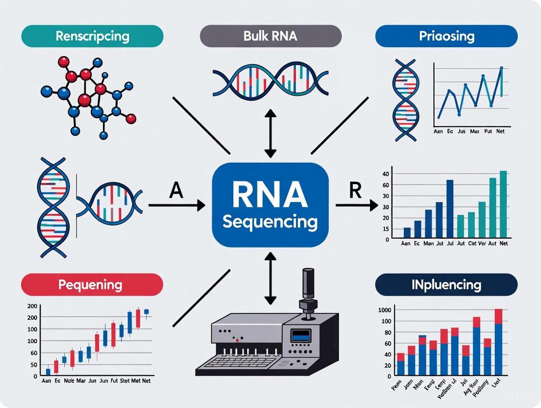
This article provides a comprehensive overview of bulk RNA sequencing for whole transcriptome analysis, tailored for researchers and drug development professionals.
Bulk RNA-Seq for Whole Transcriptome Profiling: A Comprehensive Guide from Foundations to Clinical Applications
Abstract
This article provides a comprehensive overview of bulk RNA sequencing for whole transcriptome analysis, tailored for researchers and drug development professionals. It covers foundational principles, including how bulk RNA-seq measures average gene expression across cell populations and its key advantages in cost-effectiveness and established analytical pipelines. The guide explores cutting-edge methodologies and clinical applications, from differential expression analysis with DESeq2 to biomarker discovery and therapy guidance. It addresses critical troubleshooting aspects, including normalization challenges posed by transcriptome size variation and solutions for low-quality input. Finally, it examines validation strategies and comparative analyses with emerging technologies like single-cell and spatial transcriptomics, positioning bulk RNA-seq within the modern multi-omics landscape.
Understanding Bulk RNA-Seq: Core Principles and Transcriptome Biology
What is Bulk RNA Sequencing? Defining Population-Averaged Gene Expression
Bulk RNA Sequencing (bulk RNA-seq) is a foundational next-generation sequencing (NGS) method for transcriptome profiling of pooled cell populations, tissue sections, or biopsies [1]. This technique provides a population-averaged readout, measuring the average expression level of individual genes across hundreds to millions of input cells [1] [2]. By capturing the global gene expression profile of a sample, bulk RNA-seq enables researchers to identify expression differences between experimental conditions, such as diseased versus healthy tissues, or treated versus control samples [2] [3]. Unlike later-developed single-cell methods, bulk RNA-seq generates a composite expression profile representing the entire cell population within a sample, making it invaluable for comparative transcriptomics and biomarker discovery [2].
The significance of bulk RNA-seq lies in its ability to provide a comprehensive quantitative overview of the transcriptome during specific developmental stages or physiological conditions [4]. This approach has revolutionized transcriptomics by offering a far more precise measurement of transcript levels and their isoforms compared to previous hybridization-based methods like microarrays [4]. Understanding the transcriptome is essential for interpreting the functional elements of the genome and revealing the molecular constituents of cells and tissues, which has profound implications for understanding development and disease [4].
Key Methodologies and Protocols
Standard Bulk RNA-seq Workflow
The bulk RNA-seq workflow comprises multiple critical steps, from sample preparation to sequencing, each requiring specific protocols and quality controls to ensure reliable data.
Sample Preparation and Library Construction
The process begins with RNA extraction from the biological sample, which could be total RNA or RNA enriched for specific types through poly(A) selection or ribosomal RNA depletion [1] [5]. For mRNA sequencing, Oligo(dT) is often used to enrich mRNA or deplete ribosomal RNA [2]. Assessing RNA quality is crucial before proceeding, commonly evaluated using the RNA Integrity Number (RIN), with a value over six generally considered acceptable for sequencing [5].
Following quality control, the protocol involves:
- Fragmentation of RNA into smaller pieces (200-500 bp) via enzymatic, chemical, or physical means to be compatible with sequencing platforms [4] [5]
- Reverse transcription of RNA into double-stranded cDNA [1] [5]
- Adapter ligation with platform-specific sequences to enable sequencing [4] [5]
- Sample multiplexing using unique barcodes to pool multiple samples together for efficient library preparation [1]
For projects requiring higher sensitivity with limited starting material, methods like CEL-seq2 incorporate unique barcodes to label each sample before pooling, followed by linear amplification via in vitro transcription (IVT) to generate amplified RNA [1].
Sequencing and Data Generation
The prepared libraries are sequenced using high-throughput platforms, with Illumina systems being the most common [2]. Both single-end and paired-end (PE) sequencing approaches are used, with PE recommended for differential expression analysis as it preserves strand information and provides more accurate alignment, especially for isoform studies [6] [5]. The resulting sequences, called "reads," typically range from 30-400 bp depending on the technology used [4].
Computational Analysis Pipeline
Following sequencing, computational analysis transforms raw data into biological insights through multiple processing stages.
Quality Control and Read Alignment
The initial computational steps include:
- Quality checking of sequence data using tools like FastQC to assess completeness, depth, and read quality [7]
- Adapter trimming and quality filtering with tools like Trimmomatic [7]
- Read alignment to a reference genome using splice-aware aligners such as STAR, or alignment to transcriptomes using tools like Bowtie2 [7] [6]
- Pseudoalignment approaches using tools like Salmon or kallisto that provide faster quantification without base-level alignment [6]
For gene-level quantification, alignment files are processed using tools like HTSeq-count to generate count matrices where rows represent genes and columns represent samples [7]. The nf-core/rnaseq workflow provides an automated, reproducible pipeline that integrates these steps, combining STAR alignment with Salmon quantification for optimal results [6].
Differential Expression Analysis
The count matrix serves as input for statistical analysis to identify differentially expressed genes (DEGs). Two widely used tools for this purpose are DESeq2 and limma [7] [6]. DESeq2 employs a negative binomial distribution to model count data and uses the Wald test to identify significant expression changes between conditions [7]. The analysis includes:
- Data normalization to account for differences in sequencing depth between samples [7]
- Statistical testing with multiple testing correction, typically using the Benjamini-Hochberg False Discovery Rate (FDR) to control for false positives [7]
- Effect size estimation using empirical Bayes shrinkage to prevent technical artifacts from inflating fold-change values [7]
Research Applications and Method Selection
Primary Applications of Bulk RNA-seq
Bulk RNA-seq serves multiple research purposes across various biological disciplines, with key applications including:
Differential Gene Expression Analysis: Comparing gene expression profiles between different experimental conditions to identify upregulated or downregulated genes [2] [3]. This application is fundamental for discovering RNA-based biomarkers and molecular signatures for disease diagnosis, prognosis, and stratification [3].
Tissue or Population-level Transcriptomics: Obtaining global expression profiles from whole tissues, organs, or bulk-sorted cell populations [3]. This approach is particularly valuable for large cohort studies, biobank projects, and establishing baseline transcriptomic profiles for new or understudied organisms [3].
Transcriptome Characterization: Identifying and annotating isoforms, non-coding RNAs, alternative splicing events, and gene fusions [4] [3]. Bulk RNA-seq can reveal precise transcription boundaries to single-base resolution and detect sequence variations in transcribed regions [4].
Pathway and Network Analysis: Investigating how sets of genes change collectively under various biological conditions to understand regulatory mechanisms and interactions within biological systems [2].
Table 1: Key Applications of Bulk RNA Sequencing
| Application Area | Specific Use Cases | Typical Outputs |
|---|---|---|
| Differential Expression | Disease vs. healthy tissue; Treated vs. control conditions; Time-course experiments | Lists of significantly upregulated/downregulated genes with statistical measures |
| Transcriptome Annotation | Novel transcript discovery; Alternative splicing analysis; Non-coding RNA characterization | Catalog of transcript species; Splicing patterns; Transcription start/end sites |
| Biomarker Discovery | Diagnostic and prognostic marker identification; Patient stratification signatures | Gene expression signatures with predictive value for specific conditions |
| Pathway Analysis | Biological mechanism elucidation; Drug response studies; Systems biology | Enriched pathways; Gene regulatory networks; Co-expression modules |
Comparative Analysis: Bulk RNA-seq vs. Single-Cell RNA-seq
The choice between bulk and single-cell RNA-seq depends on research objectives, budget, and sample characteristics, as each approach offers distinct advantages and limitations.
Table 2: Bulk RNA-seq vs. Single-Cell RNA-seq Comparison
| Aspect | Bulk RNA Sequencing | Single-Cell RNA Sequencing |
|---|---|---|
| Resolution | Population-averaged gene expression | Individual cell gene expression |
| Sample Input | RNA extracted from cell populations | Viable single-cell suspensions |
| Cost | Relatively low | Higher |
| Data Complexity | Simplified analysis | Complex data requiring specialized analysis |
| Ideal Applications | Differential expression between conditions; Large cohort studies | Cellular heterogeneity; Rare cell populations; Developmental trajectories |
| Limitations | Masks cellular heterogeneity; Cannot identify novel cell types | Higher technical noise; More complex sample preparation |
Bulk RNA-seq provides a cost-effective approach for whole transcriptome analysis with lower sequencing depth requirements and more straightforward data analysis [3]. However, its primary limitation is the inability to resolve cellular heterogeneity, as it averages expression across all cells in a sample [2] [3]. This means bulk RNA-seq cannot identify rare cell types or distinguish whether expression signals originate from all cells or a specific subset [3].
In contrast, single-cell RNA-seq enables resolution of cellular heterogeneity and identification of novel cell types and states, but requires more complex sample preparation, deeper sequencing, and specialized computational analysis [2] [3]. For many research questions, particularly those focused on population-level differences rather than cellular heterogeneity, bulk RNA-seq remains the most practical and informative choice [3].
Essential Research Reagents and Tools
Successful bulk RNA-seq experiments require specific reagents, tools, and computational resources throughout the workflow.
Table 3: Essential Research Reagent Solutions for Bulk RNA-seq
| Category | Specific Tools/Reagents | Function/Purpose |
|---|---|---|
| RNA Extraction & QC | TRIzol; PicoPure RNA Isolation Kit; Qubit; Agilent TapeStation | RNA isolation and quality assessment; Concentration determination |
| Library Preparation | Oligo(dT) beads; rRNA depletion kits; NEBNext Ultra DNA Library Prep Kit | mRNA enrichment; cDNA synthesis; Adapter ligation |
| Sequencing | Illumina platforms; SOLiD; Roche 454 | High-throughput sequencing of cDNA libraries |
| Alignment & Quantification | STAR; HISAT2; Salmon; kallisto; HTSeq-count | Read alignment to reference; Gene-level quantification |
| Differential Expression | DESeq2; limma; edgeR | Statistical analysis of expression differences |
| Visualization & Interpretation | PCA; Heatmaps; Volcano plots; WGCNA; GSEA | Data exploration; Pattern identification; Biological interpretation |
Key considerations for reagent selection include:
- RNA quality assessment tools are essential, with RIN values >6 recommended for sequencing [5]
- Strand-specific library preparation protocols preserve transcript orientation information, valuable for transcriptome annotation [4]
- Multiplexing barcodes enable efficient processing of multiple samples in a single sequencing run [1]
- Reference genomes and annotation files (GTF/GFF) must match the target organism for accurate alignment and quantification [7] [6]
The integration of these tools within automated workflows, such as the nf-core/rnaseq pipeline, enhances reproducibility and efficiency in bulk RNA-seq analysis [6]. This workflow combines optimal tools at each step, from STAR alignment to Salmon quantification and DESeq2 differential expression analysis, providing researchers with a standardized approach to transcriptome profiling [6].
In bulk RNA sequencing (RNA-seq), the pervasive presence of ribosomal RNA (rRNA)—constituting 80-90% of total RNA—poses a significant challenge to transcriptome analysis [8] [9]. To overcome this, two principal library preparation strategies have been developed: poly(A) enrichment and rRNA depletion. The choice between these methods represents a critical, irreversible decision that determines which RNA molecules enter the sequencing library, directly impacting data quality, experimental cost, and the biological conclusions that can be drawn [8]. Poly(A) enrichment selectively targets polyadenylated transcripts through oligo(dT) hybridization, making it ideal for profiling mature messenger RNAs (mRNAs) in eukaryotes. In contrast, rRNA depletion employs sequence-specific probes to remove abundant rRNAs from total RNA, preserving both polyadenylated and non-polyadenylated RNA species [8] [10]. This application note details the technological features of both methods, providing structured comparisons, detailed protocols, and decision frameworks to guide researchers in selecting the optimal approach for their specific experimental contexts within whole transcriptome profiling research.
Core Principles and Molecular Mechanisms
Poly(A) Enrichment: A Targeted Capture Approach
The poly(A) enrichment method operates on the principle of oligo(dT) hybridization to capture RNAs possessing a poly(A) tail. This process utilizes oligo(dT) primers or probes conjugated to magnetic beads, which selectively bind to the poly(A) tails of mature eukaryotic mRNAs and many long non-coding RNAs (lncRNAs) [8] [10]. During library preparation, total RNA is incubated with these beads, allowing the poly(A)+ RNAs to hybridize. Subsequent washing steps remove non-polyadenylated RNAs, including the majority of rRNAs, transfer RNAs (tRNAs), and small nuclear RNAs (snRNAs). The captured poly(A)+ RNA is then eluted and serves as the input for downstream library construction [10]. This mechanism effectively enriches for protein-coding transcripts while excluding non-polyadenylated species such as replication-dependent histone mRNAs and many non-coding RNAs [8]. A key consideration is that the efficiency of this capture depends heavily on an intact poly(A) tail, making the method susceptible to performance degradation with RNA samples that are partially degraded or fragmented, as is common with formalin-fixed paraffin-embedded (FFPE) samples [8] [11].
rRNA Depletion: A Subtraction-Based Strategy
rRNA depletion employs a subtraction-based methodology designed to remove abundant ribosomal RNAs from total RNA, thereby enriching for all other RNA species. This is typically achieved using sequence-specific DNA or LNA (Locked Nucleic Acid) probes that are complementary to the rRNA sequences of the target organism (e.g., 18S and 28S rRNAs in eukaryotes) [8] [9]. These probes hybridize to their target rRNAs, and the resulting probe-rRNA hybrids are subsequently removed from the solution. Removal can be accomplished through several mechanisms, including immobilization on magnetic beads (e.g., streptavidin-beads if the probes are biotinylated) or enzymatic degradation via RNase H, which specifically cleaves RNA in RNA-DNA hybrids [8]. The remaining supernatant, now depleted of rRNA, contains a diverse pool of both poly(A)+ and non-polyadenylated RNAs, including pre-mRNAs, many lncRNAs, histone mRNAs, and some viral RNAs [8] [10]. This method does not rely on the presence of a poly(A) tail, making it notably more resilient when working with fragmented RNA from FFPE or other compromised samples [8] [12].
Comparative Technical Performance and Data Characteristics
The choice between poly(A) enrichment and rRNA depletion profoundly impacts the composition and quality of the resulting sequencing data, influencing everything from read distribution to required sequencing depth and analytical complexity. Understanding these technical differences is paramount for experimental design and data interpretation.
Table 1: Performance Characteristics of Poly(A) Enrichment vs. rRNA Depletion
| Performance Metric | Poly(A) Enrichment | rRNA Depletion | Experimental Implications |
|---|---|---|---|
| Usable Exonic Reads | 70-71% [10] | 22-46% [10] | Poly(A) yields more mRNA data per sequencing dollar |
| Sequencing Depth Required | Lower (Baseline) | 50-220% higher [10] | Higher cost for equivalent exonic coverage with depletion |
| Transcript Types Captured | Mature, polyadenylated mRNA | Coding + non-coding RNA (lncRNA, pre-mRNA) [8] [10] | Depletion enables discovery of non-poly(A) transcripts |
| Read Distribution (Bias) | Pronounced 3' bias [8] [11] | More uniform 5'-to-3' coverage [11] | Depletion better for isoform/splice analysis |
| Genomic Feature Mapping | High exonic, low intronic [11] | Lower exonic, high intronic/intergenic [8] [11] | Intronic reads in depletion can indicate nascent transcription |
| Performance with FFPE/Degraded RNA | Poor; strong 3' bias, low yield [8] [12] | Robust; tolerates fragmentation [8] [12] | Depletion is the standard for clinical/archival samples |
| Residual rRNA Content | Very Low [11] | Low, but variable (probe-dependent) [8] [9] | Verify probe match for non-model organisms |
The data characteristics extend beyond simple metrics. Poly(A) selection, by focusing on mature mRNAs, removes most intronic and intergenic sequences, leading to a high fraction of reads mapping to annotated exons. This improves statistical power for gene-level differential expression analysis at a given sequencing depth [8]. In contrast, rRNA depletion retains a broader spectrum of RNA species, resulting in increased intronic and intergenic fractions. While this can initially appear as "noise," this "extra" signal is often biologically informative; for instance, intronic reads can track transcriptional changes, while exonic reads integrate post-transcriptional processing, allowing researchers to separate these regulatory mechanisms when modeled together [8]. Furthermore, a study comparing library protocols for FFPE samples found that rRNA depletion methods (e.g., Illumina Stranded Total RNA Prep) can preserve a high percentage of reads mapping to intronic regions (~60%), underscoring their ability to capture pre-mRNA and nascent transcription [12].
Detailed Methodologies and Experimental Protocols
Protocol for Poly(A) Enrichment and Library Construction
Principle: Utilize oligo(dT)-conjugated magnetic beads to isolate polyadenylated RNA from total RNA [8] [10].
- Starting Material: 10-1000 ng of high-quality total RNA (RIN ≥ 7 or DV200 ≥ 50% is recommended) [8].
- Key Reagents: Oligo(dT) magnetic beads, Binding Buffer, Wash Buffer, Nuclease-free Water.
Procedure: 1. RNA Denaturation: Heat the total RNA sample to 65°C for 2 minutes and immediately place on ice. This disrupts secondary structures. 2. Binding: Combine the denatured RNA with oligo(dT) beads in a high-salt binding buffer. Incubate at room temperature for 5-10 minutes with gentle agitation. The salt condition promotes hybridization between the poly(A) tail and the oligo(dT) matrices. 3. Capture and Wash: Place the tube on a magnetic stand to separate the beads from the supernatant. Carefully remove and discard the supernatant, which contains non-polyadenylated RNA (rRNA, tRNA, etc.). 4. Washing: Wash the bead-bound poly(A)+ RNA twice with a low-salt wash buffer without disturbing the pellet. This step removes weakly associated and non-specifically bound RNAs. 5. Elution: Elute the purified poly(A)+ RNA from the beads using nuclease-free water or Tris buffer by heating to 70-80°C for 2 minutes. 6. Library Construction: Proceed with standard stranded RNA-seq library prep protocols (fragmentation, reverse transcription, adapter ligation, and PCR amplification) using the eluted poly(A)+ RNA as input.
Optimization Note: For challenging samples or non-standard organisms, the beads-to-RNA ratio may require optimization. Recent research on yeast RNA showed that increasing the oligo(dT) beads-to-RNA ratio significantly reduced residual rRNA content, and a second round of enrichment could further improve purity, though at the cost of yield [9].
Protocol for rRNA Depletion and Library Construction
Principle: Use species-specific DNA probes complementary to rRNA to hybridize and remove rRNA from total RNA [8] [12].
- Starting Material: 10-1000 ng of total RNA. Integrity requirements are flexible (compatible with RIN < 7 and FFPE RNA) [8] [12].
- Key Reagents: rRNA-targeted DNA/LNA probes (e.g., Ribo-Zero/Ribo-Gone), Hybridization Buffer, RNase H (optional), Magnetic Beads for capture.
Procedure: 1. Hybridization: Mix total RNA with the biotinylated rRNA-depletion probes in a hybridization buffer. Incubate the mixture at a defined temperature (e.g., 68°C) for 10-30 minutes to allow the probes to bind specifically to their target rRNA sequences. 2. Removal of rRNA-Probe Hybrids: * Bead Capture Method: Add streptavidin-coated magnetic beads to the mixture. Incubate to allow the biotinylated probes (hybridized to rRNA) to bind to the beads. Use a magnetic stand to capture the beads, and transfer the supernatant—now depleted of rRNA—to a new tube [8] [11]. * Enzymatic Digestion Method: After hybridization, add RNase H to the mixture. This enzyme cleaves the RNA strand in RNA-DNA hybrids, specifically digesting the rRNA bound to the DNA probes. The reaction is then cleaned up to remove fragments and enzymes [8]. 3. Clean-up: Purify the rRNA-depleted RNA using a standard RNA clean-up protocol (e.g., ethanol precipitation or solid-phase reversible immobilization beads). 4. Library Construction: The resulting rRNA-depleted RNA (total transcriptome) is used as input for stranded RNA-seq library prep, which typically involves random priming for cDNA synthesis to ensure uniform coverage across transcripts.
Critical Consideration: The efficiency of depletion is highly dependent on the complementarity between the probes and the target rRNA sequences. For non-model organisms, it is crucial to verify probe match, as mismatches can lead to high residual rRNA and wasted sequencing reads [8].
Decision Framework and Application Guidelines
Selecting the appropriate RNA-seq library preparation method is a strategic decision that hinges on three primary filters: the organism, RNA integrity, and the biological question regarding target RNA species [8]. The following structured framework guides this selection process.
Table 2: Method Selection Guide Based on Experimental Context
| Experimental Context | Recommended Method | Rationale | Technical Considerations |
|---|---|---|---|
| Eukaryotic, High-Quality RNA (RIN ≥8), mRNA Focus | Poly(A) Selection [8] [10] | Maximizes exonic reads & power for differential expression | Coverage skews to 3' if integrity is suboptimal [8] |
| Degraded/FFPE RNA, Clinical Archives | rRNA Depletion [8] [10] [12] | Does not rely on intact poly(A) tails; more robust | Intronic fractions rise; confirm RNA quality (DV200) [12] |
| Prokaryotic Transcriptomics | rRNA Depletion [8] | Poly(A) capture is not appropriate for bacteria | Use species-matched rRNA probes |
| Non-Coding RNA Discovery | rRNA Depletion [8] [10] | Retains non-polyadenylated RNAs (lncRNAs, snoRNAs) | Residual rRNA increases if probes are off-target |
| Need for Nascent Transcription | rRNA Depletion [8] | Captures pre-mRNA and intronic sequences | Model intronic and exonic reads jointly |
| Cost-Sensitive, High-Throughput mRNA Quantification | Poly(A) Selection [10] [13] | Lower sequencing depth required; simpler analysis | 3' mRNA-Seq (e.g., QuantSeq) is a specialized option [13] |
The decision matrix can be further visualized through a simple workflow. It is critical to maintain methodological consistency; once a strategy is chosen for a study, it should be kept constant for all samples to ensure comparability of results [8].
The Scientist's Toolkit: Essential Research Reagents and Kits
Successful implementation of poly(A) enrichment or rRNA depletion requires specific reagent systems. The following table catalogs key solutions and their functions as derived from the literature and commercial platforms.
Table 3: Key Research Reagent Solutions for RNA-seq Library Preparation
| Reagent / Kit Name | Function | Key Features / Applications | Technical Notes |
|---|---|---|---|
| Oligo(dT) Magnetic Beads [10] [9] | Poly(A)+ RNA selection | Basis of most poly(A) enrichment protocols; available from multiple vendors (e.g., NEB, Invitrogen) | Beads-to-RNA ratio is a key optimization parameter [9] |
| Poly(A)Purist MAG Kit [9] | Poly(A)+ RNA selection | Commercial kit with optimized buffers for purification | |
| Ribo-Zero Plus [12] | rRNA depletion | Used in Illumina Stranded Total RNA Prep; effective for FFPE RNA [12] | Shows very low residual rRNA (~0.1%) in studies [12] |
| RiboMinus Kit [9] | rRNA depletion | Uses LNA probes for efficient hybridization and removal | Probe specificity is critical for performance |
| SMARTer Stranded Total RNA-Seq Kit [12] | rRNA depletion & library prep | All-in-one kit; performs well with low RNA input (e.g., FFPE) [12] | Can have higher residual rRNA than other methods; requires deeper sequencing [12] |
| Duplex-Specific Nuclease (DSN) [11] | rRNA depletion | Normalizes transcripts by digesting abundant ds-cDNA (from rRNA) | Can show higher variability and intronic mapping [11] |
| QuantSeq 3' mRNA-Seq Kit [13] | 3'-focused mRNA sequencing | Ultra-high-throughput, cost-effective for gene counting | Ideal for large-scale screening; simpler analysis [13] |
Poly(A) enrichment and rRNA depletion are both powerful but distinct strategies for preparing RNA-seq libraries. Poly(A) enrichment remains the gold standard for efficient, cost-effective profiling of mature mRNA from high-quality eukaryotic samples, delivering a high fraction of usable exonic reads. In contrast, rRNA depletion offers unparalleled flexibility, enabling transcriptome-wide analysis that includes non-coding RNAs, pre-mRNAs, and transcripts from degraded clinical samples or prokaryotes. The decision is not one of superiority but of appropriateness. By carefully considering the organism, sample quality, and biological question—and by leveraging the decision frameworks and protocols outlined herein—researchers can confidently select the optimal method to ensure the success and biological relevance of their whole transcriptome profiling research.
The Biological Significance of Transcriptome Size Variation Across Cell Types
In the field of bulk RNA-seq research, a critical biological variable often overlooked in experimental design and data analysis is transcriptome size—the total number of RNA molecules within an individual cell. Different cell types inherently possess different transcriptome sizes, a feature rooted in their biological identity and function [14] [15]. For instance, a red blood cell, specialized for oxygen transport, predominantly expresses hemoglobin transcripts, whereas a pluripotent stem cell may express thousands of different genes to maintain its undifferentiated state [15]. This variation is not merely a biological curiosity; it presents a substantial challenge for the accurate interpretation of bulk RNA-seq data, which measures the averaged gene expression from a potentially heterogeneous mixture of cells [14].
Traditional bioinformatics practices, particularly normalization methods, frequently operate on the assumption that transcriptome size is constant across cell types. Commonly used techniques like Counts Per Million (CPM) or Counts Per 10 Thousand (CP10K) effectively eliminate technology-derived effects but simultaneously remove the genuine biological variation in transcriptome size [14]. This creates a systematic scaling effect that can distort biological interpretation, especially in experiments involving diverse cell populations, such as those found in complex tissues or the tumor microenvironment [14] [16]. This review details the biological significance of transcriptome size variation and introduces emerging methodologies and tools designed to account for this factor, thereby enhancing the accuracy of bulk RNA-seq analysis.
Biological Foundations and Quantitative Evidence
Transcriptome size variation is a consistent and measurable feature across different cell types. Evidence from comprehensive single-cell atlases, such as those of the mouse and human cortex, confirms that while cells of the same type typically exhibit similar transcriptome sizes, this size can vary significantly—often by multiple folds—across different cell types [14] [17]. For example, an analysis of mouse specimens showed that the average transcriptome size of L5 PT CTX cells was approximately 21.6k in one sample but increased to 31.9k in another, indicating that variation can exist for the same cell type across different specimens or conditions [14].
The biological implications of this diversity are profound. A study profiling 91 cells from five mouse tissues found that pyramidal neurons exhibited significantly greater transcriptome complexity, with an average of 14,964 genes expressed per cell, compared to an average of 7,939 genes in brown adipocytes, cardiomyocytes, and serotonergic neurons [17]. This broad transcriptional repertoire in neurons is thought to underpin their high degree of phenotypic plasticity, a stark contrast to the more specialized and narrower functional repertoire of heart and fat cells [17]. Furthermore, transcriptome diversity, quantified using Shannon entropy, has been identified as a major systematic source of variation in RNA-seq data, strongly correlating with the expression of most genes and often representing the primary component identified by factor analysis tools [18].
Table 1: Documented Transcriptome Size and Complexity Across Mammalian Cell Types
| Cell Type | Tissue/Origin | Key Metric | Approximate Value | Biological Implication |
|---|---|---|---|---|
| Pyramidal Neurons | Mouse Cortex/Hippocampus | Number of Expressed Genes [17] | ~15,000 genes/cell | Underpins phenotypic plasticity and complex function. |
| Non-Neuronal Cells (Cardiomyocytes, Brown Adipocytes) | Mouse Heart/Fat | Number of Expressed Genes [17] | ~8,000 genes/cell | Reflects a narrower, more specialized functional role. |
| L5 PT CTX Neurons | Mouse Cortex (Sample I) | Total Transcriptome Size [14] | ~21,600 molecules/cell | Indicates biological variation within a specific cell type across specimens. |
| L5 PT CTX Neurons | Mouse Cortex (Sample II) | Total Transcriptome Size [14] | ~31,900 molecules/cell | Indicates biological variation within a specific cell type across specimens. |
Impact on Bulk RNA-Seq Analysis and Deconvolution
In bulk RNA-seq, the signal is an aggregate from potentially millions of cells. When these cells have intrinsically different transcriptome sizes, standard normalization distorts the true biological picture. The scaling effect introduced by CP10K normalization enlarges the relative expression profile of cell types with smaller transcriptomes and shrinks those with larger ones [14]. This is particularly problematic for cellular deconvolution, the computational process of inferring cell type proportions from bulk RNA-seq data using single-cell RNA-seq (scRNA-seq) data as a reference.
When a CP10K-normalized scRNA-seq reference is used for deconvolution, the scaling effect leads to significant inaccuracies. Cell types with smaller true transcriptome sizes, which are often rare cell populations like certain immune cells in a tumor microenvironment, have their proportions systematically underestimated because their expression profiles were artificially inflated during normalization [14] [15]. Furthermore, two other critical issues compound this problem: the gene length effect, where bulk RNA-seq counts are influenced by gene length (an effect absent from UMI-based scRNA-seq), and the expression variance, where the natural variation in gene expression within a cell type is not properly modeled [14]. Failure to address these three issues results in biased deconvolution outcomes that can mislead downstream biological interpretations.
Protocols and Methodologies
Experimental Protocol: Bulk RNA-Seq Library Preparation with BOLT-seq
For large-scale transcriptome profiling where cost and throughput are primary concerns, the BOLT-seq (Bulk transcriptOme profiling of cell Lysate in a single poT) protocol offers a highly scalable and cost-effective solution (estimated at <$1.40 per sample) [19].
1. Principle: BOLT-seq is a 3'-end mRNA-seq method that constructs sequencing libraries directly from crude cell lysates without requiring RNA purification, significantly reducing hands-on time and steps. It uses in-house purified enzymes to further lower costs [19].
2. Reagents and Equipment:
- Cells: Up to 1,000 cells per sample in a 96-well microtiter plate.
- Lysis Buffer: Contains 0.3% IGEPAL CA-630.
- Enzymes: In-house purified M-MuLV Reverse Transcriptase and Tn5 Transposase.
- Primers: Anchored oligo(dT)30-P7 RT primer.
- Reaction Buffers: RT-Mix-B, TD-Mix, PCR-Mix.
- Thermal Cycler
3. Step-by-Step Procedure:
- Step 1: Cell Lysis. Seed cells in a 96-well plate. Wash with DPBS and lyse with 60 µL of lysis buffer. Incubate for 30 minutes with shaking at 800 RPM.
- Step 2: RNA Denaturation. Transfer 6 µL of cell lysate to a PCR tube. Add 1 µL of RT-Mix-A (containing the anchored oligo(dT) RT primer and dNTPs). Incubate at 65°C for 5 minutes, then immediately place on ice for 3 minutes.
- Step 3: Reverse Transcription. Add 7 µL of RT-Mix-B (containing reaction buffer, DTT, PEG8000, RNase inhibitor, and M-MuLV RT). Incubate at 50°C for 60 minutes. Inactivate the reaction at 80°C for 10 minutes. No purification is needed.
- Step 4: Tagmentation. Add 5 µL of TD-Mix (containing reaction buffer, PEG8000, tetraethylene glycol, and Tn5 transposase) to the RNA/DNA hybrid duplexes. Incubate at 55°C for 30 minutes. Stop the reaction by adding 5 µL of 0.2% SDS. No purification is needed.
- Step 5: Gap-Filling and PCR Amplification. Add 25 µL of PCR-Mix (containing HiFi Fidelity Buffer, dNTPs, HiFi HotStart DNA Polymerase, and indexed primers). Perform the following program in a thermal cycler:
- 50°C for 10 minutes (Gap-filling)
- 95°C for 3 minutes (Initial denaturation)
- 18 cycles of: 95°C for 30s, 60°C for 30s, 72°C for 30s
- 72°C for 3 minutes (Final extension)
- The final libraries can be purified and sequenced on a platform such as Illumina's NovaSeq 6000 [19].
BOLT-seq Workflow: A simplified protocol for cost-effective, high-throughput 3' mRNA-seq.
Computational Protocol: Accurate Deconvolution with ReDeconv
The ReDeconv computational framework is specifically designed to address the pitfalls of transcriptome size variation in deconvolution analysis [14] [15].
1. Principle: ReDeconv introduces a novel normalization method for scRNA-seq reference data that preserves true transcriptome size differences, corrects for gene length effects in bulk data, and incorporates gene expression variance into its model [14].
2. Software and Inputs:
- Tool: ReDeconv (Available at https://redeconv.stjude.org).
- Input 1: Raw count matrix from scRNA-seq data (reference).
- Input 2: Bulk RNA-seq data (mixture).
- Environment: Computational environment with R/Python as required.
3. Step-by-Step Procedure:
- Step 1: scRNA-seq Reference Normalization. Normalize the raw scRNA-seq count data using the CLTS (Count based on Linearized Transcriptome Size) method instead of CP10K. This step preserves the inherent biological variation in transcriptome size across different cell types in the reference.
- Step 2: Bulk Data Normalization. Apply TPM (Transcripts Per Million) or RPKM/FPKM normalization to the bulk RNA-seq data. This step specifically mitigates the gene length effect that is present in bulk protocols but not in UMI-based scRNA-seq.
- Step 3: Signature Gene Selection. For each cell type in the reference, identify and use a set of signature genes that exhibit stable expression with low variance. This leverages the single-cell resolution of the reference to improve the robustness of the deconvolution model.
- Step 4: Deconvolution Modeling. Execute the ReDeconv algorithm, which integrates the normalized reference and bulk data, along with the variance-stabilized signature genes, to estimate cell type proportions in the bulk sample. The model is designed to be particularly sensitive to rare cell types [14] [15].
ReDeconv Analysis Workflow: A computational pipeline correcting for transcriptome size, gene length, and expression variance.
Table 2: Key Research Reagents and Computational Tools for Transcriptome Size-Aware Analysis
| Item Name | Type | Function/Application | Key Feature |
|---|---|---|---|
| BOLT-seq Reagents [19] | Wet-lab Protocol | Cost-effective 3'-end mRNA-seq library prep from cell lysates. | Eliminates RNA purification; single-tube reaction; very low cost per sample. |
| In-house Tn5 Transposase [19] | Laboratory Reagent | Enzyme for tagmentation step in BOLT-seq. | Custom purified, significantly reduces library preparation costs. |
| ReDeconv [14] [15] | Computational Tool/Algorithm | Improved scRNA-seq normalization and bulk RNA-seq deconvolution. | Incorporates transcriptome size, gene length effect, and expression variance. |
| CLTS Normalization [14] | Computational Method | Normalization for scRNA-seq data within ReDeconv. | Preserves biological variation in transcriptome size across cell types. |
| Stranded mRNA Prep Kits (e.g., Illumina) [20] | Commercial Kit | Standard whole-transcriptome or mRNA-seq library preparation. | Determines transcript strand of origin; high sensitivity and dynamic range. |
| Salmon [6] | Computational Tool | Alignment-free quantification of transcript abundance from RNA-seq data. | Handles read assignment uncertainty rapidly; integrates well with workflows like nf-core/rnaseq. |
Transcriptome size variation is a fundamental biological feature with profound implications for the accuracy of bulk RNA-seq analysis. Ignoring this factor, especially in studies of heterogeneous tissues, introduces a systematic bias that compromises the identification of differentially expressed genes and the estimation of cellular abundances. The integration of next-generation experimental protocols like BOLT-seq with sophisticated computational frameworks like ReDeconv, which explicitly models biological parameters such as transcriptome size, represents a critical advancement. By adopting these tools and methodologies, researchers can unlock more precise and biologically meaningful insights from their transcriptomic data, thereby enhancing discoveries in fields ranging from developmental biology to cancer research.
Bulk RNA-seq remains a cornerstone technique for whole transcriptome profiling, providing a population-average view of gene expression. This averaging effect is a fundamental characteristic that presents both a key advantage and a significant inherent limitation. While it offers a robust, cost-efficient overview of the transcriptional state of a tissue or cell population, it simultaneously masks the underlying cellular heterogeneity. For researchers and drug development professionals, understanding this duality is critical for designing experiments, interpreting data, and selecting the appropriate tool for their biological questions. This application note details the implications of the population averaging effect and provides methodologies to overcome its limitations.
The Principle of Population Averaging
In bulk RNA sequencing, the starting material consists of RNA extracted from a population of thousands to millions of cells. The resulting sequencing library represents a pooled transcriptome, where the expression level for each gene is measured as an average across all cells in the sample [5] [3]. This provides a composite profile, effectively homogenizing the contributions of individual cells.
The following diagram illustrates the fundamental workflow of bulk RNA-seq and where the population averaging occurs.
Advantages: The Power of an Average
The population-level view conferred by bulk RNA-seq offers several distinct advantages for whole transcriptome research, as outlined in the table below.
Table 1: Key Advantages of the Population Averaging Effect in Bulk RNA-seq
| Advantage | Description | Common Applications |
|---|---|---|
| Holistic Profiling | Provides a global, averaged expression profile from whole tissues or organs, representing the collective biological state [3]. | Establishing baseline transcriptomic profiles for tissues; large cohort studies and biobanks [3]. |
| Cost-Efficiency & Simplicity | Lower per-sample cost and simpler sample preparation compared to single-cell methods [3]. | Pilot studies; powering experiments with high numbers of biological replicates. |
| High Sensitivity for Abundant Transcripts | Effective detection and quantification of medium to highly expressed genes due to the large amount of input RNA. | Differential gene expression analysis between conditions (e.g., disease vs. healthy) [3]. |
| Comprehensive Transcriptome Characterization | Can be used to annotate isoforms, non-coding RNAs, alternative splicing events, and gene fusions from a deep sequence of the transcriptome [3] [21]. | Discovery of novel transcripts and biomarker signatures [21]. |
Inherent Limitations: The Consequences of Averaging
The primary limitation of population averaging is its inability to resolve cellular heterogeneity. This can lead to several specific challenges and potential misinterpretations of data.
Table 2: Key Limitations Arising from the Population Averaging Effect
| Limitation | Consequence | Practical Example |
|---|---|---|
| Masking of Cell-Type-Specific Expression | Gene expression changes unique to a rare or minority cell population are diluted and may go undetected [5] [3]. | A transcript upregulated in a rare stem cell population (e.g., <5% of cells) may not appear significant in a bulk profile. |
| Obfuscation of Cellular Heterogeneity | Cannot distinguish between a uniform change in gene expression across all cells versus a dramatic change in a specific subpopulation [21]. | An apparent two-fold increase in a bulk sample could mean a small change in all cells, or a 100-fold change in just 2% of cells. |
| Inability to Identify Novel Cell Types/States | The averaged profile cannot reveal the existence of previously uncharacterized or transient cell states within a sample [3]. | Novel immune cell activation states or rare tumor-initiating cells remain hidden. |
| Confounding by Variable Cell Type Composition | Observed differential expression between samples may be driven by differences in the proportions of constituent cell types rather than true regulatory changes within a specific lineage [22] [23]. | A disease-associated gene signature may simply reflect increased immune cell infiltration rather than altered gene expression in parenchymal cells. |
The following diagram conceptualizes how a bulk RNA-seq experiment interprets a signal from a complex, heterogeneous tissue.
Experimental Protocols to Overcome Limitations
Protocol: Computational Deconvolution of Bulk RNA-seq Data
Computational deconvolution leverages single-cell RNA-seq (scRNA-seq) reference datasets to estimate the cellular composition and cell-type-specific gene expression from bulk RNA-seq data [22] [23]. This protocol outlines the key steps.
Key Reagent Solutions for Deconvolution Analysis
Table 3: Essential Tools for Computational Deconvolution
| Research Reagent / Tool | Function | Example / Note |
|---|---|---|
| High-Quality scRNA-seq Reference | Provides the cell-type-specific gene expression signatures required for deconvolution. | Public datasets from consortia like the Human Cell Atlas [22]. Must encompass expected cell types in the bulk tissue [23]. |
| Deconvolution Algorithm | A computational method that performs the regression of bulk data onto the reference signature matrix. | Methods include SCDC [22], MuSiC [22], and Bisque [22]. SCDC is unique in its ability to integrate multiple references. |
| Bulk RNA-seq Dataset | The target dataset to be deconvoluted, comprising RNA-seq data from complex tissue samples. | Requires standard bulk RNA-seq processing: quality control, adapter trimming, and gene quantification. |
| Computational Environment | Software and hardware for running analysis, typically using R or Python. | R packages like SCDC [22] or Seurat [23] facilitate the analysis. |
Methodology:
- Acquire and Curate a scRNA-seq Reference Dataset: Obtain a publicly available or in-house scRNA-seq dataset of the same or biologically similar tissue. Critically, this reference must contain all the major cell populations expected to be present in the bulk tissue [23]. Perform standard scRNA-seq quality control and annotation to assign cell type labels to each cluster.
- Construct a Signature Matrix: From the curated scRNA-seq data, generate a cell-type-specific gene expression signature matrix. This matrix contains the average expression levels of a set of informative genes (often marker genes) across each defined cell type [22] [23].
- Apply a Deconvolution Algorithm: Input the bulk RNA-seq data and the signature matrix into a deconvolution tool. For example, the SCDC method uses an ENSEMBLE framework to integrate results from multiple scRNA-seq references, implicitly addressing batch effects and improving accuracy [22].
- Output and Validation: The algorithm outputs the estimated proportion of each cell type in every bulk sample. These results should be validated against known biological expectations or orthogonal methods like flow cytometry, if available [22].
The workflow for this deconvolution approach is detailed below.
Protocol: Interrogating Cell-Type-Specific Gene Signatures
This protocol, adapted from Cid et al., leverages existing scRNA-seq data to deconvolve patterns of cell-type-specific expression from lists of differentially expressed genes (DEGs) obtained from bulk RNA-seq [23].
Methodology:
- Generate Bulk RNA-seq DEG List: Perform a standard differential expression analysis on your bulk RNA-seq data from heterogeneous tissue to identify a list of significant DEGs between conditions.
- Map DEGs to a scRNA-seq Dataset: Extract the expression values for the identified DEGs from a curated scRNA-seq reference dataset.
- Analyze Expression Patterns: Use linear dimensionality reduction (e.g., PCA) and hierarchical clustering on the scRNA-seq data, but subset to only the DEGs from the bulk experiment. This reveals which of the bulk-derived DEGs are co-expressed in specific cell types within the reference data [23].
- Infer Biological Meaning: Identify clusters of genes that are specific to certain cell types. This can reveal whether the bulk differential expression signal is driven by changes in gene regulation within a cell type, changes in cell type abundance, or a combination of both [23].
The population averaging effect of bulk RNA-seq is an intrinsic property that defines its utility. It is a powerful tool for obtaining a quantitative, global overview of gene expression in a tissue, making it ideal for differential expression analysis in well-defined systems and large-scale cohort studies. However, in complex, heterogeneous tissues, this averaging becomes a critical limitation that can obscure biologically significant events occurring in specific cell subpopulations. By understanding these constraints and employing complementary strategies like computational deconvolution and the integration of single-cell reference data, researchers can extract deeper, more accurate insights from their bulk RNA-seq experiments, ultimately advancing discovery in basic research and drug development.
Sequencing Depth and Read Length Requirements for Different Study Goals
In bulk RNA sequencing (RNA-Seq), careful selection of sequencing depth (total number of reads per sample) and read length is fundamental to generating statistically powerful and biologically meaningful data. These parameters are not one-size-fits-all; they are dictated by the specific goals of the study, the organism's transcriptome complexity, and practical considerations of cost and time [24] [25]. Optimal experimental design ensures that the chosen depth and length provide sufficient sensitivity to detect the biological signals of interest without incurring unnecessary expenditure [26] [27]. This guide outlines evidence-based recommendations for these parameters across common research scenarios in whole transcriptome profiling, providing a framework for researchers to design robust and cost-effective RNA-Seq experiments.
Sequencing Depth Recommendations by Study Goal
Sequencing depth directly influences the sensitivity of an RNA-Seq experiment, determining the ability to detect and quantify both highly expressed and low-abundance transcripts [24] [26]. The following table summarizes the recommended sequencing depths for various research aims.
Table 1: Recommended Sequencing Depth for Different Bulk RNA-Seq Goals
| Study Goal | Recommended Sequencing Depth (Million Mapped Reads) | Key Rationale and Notes |
|---|---|---|
| Targeted RNA Expression / Focused Gene Panels | 3 - 5 million [24] | Fewer reads are required as the analysis is restricted to a pre-defined set of genes. |
| Differential Gene Expression (DGE) - Snapshot | 5 - 25 million [24] | Sufficient for a reliable snapshot of highly and moderately expressed genes [26]. |
| Standard DGE - Global View | 20 - 60 million [24] [25] | A common range for most studies; provides a more comprehensive view of expression and some capability for alternative splicing analysis [24] [28]. |
| In-depth Transcriptome Analysis | 100 - 200 million [24] | Necessary for detecting lowly expressed genes, novel transcript assembly, and detailed isoform characterization [24]. |
| Diagnostic RNA-Seq (e.g., Mendelian disorders) | 50 - 150 million [29] | Enhances diagnostic yield; deeper sequencing (e.g., >150M) can further improve detection of low-abundance pathogenic transcripts [29]. |
| Small RNA Analysis (e.g., miRNA-Seq) | 1 - 5 million [24] | Due to the small size and limited complexity of the small RNA transcriptome, fewer reads are needed. |
The Critical Role of Biological Replicates
It is crucial to recognize that sequencing depth is not the only determinant of statistical power. For differential expression analysis, the number of biological replicates (independent biological samples per condition) is often more critical than simply sequencing deeper [25] [26]. A well-powered experiment must strike a balance between depth and replication.
- Minimum Replicates: At least 3 biological replicates per condition are considered the minimum standard for statistical rigor, though 4 or more is optimal [25] [28]. Experiments with only 2 replicates have a greatly reduced ability to estimate biological variability and control false discovery rates [25].
- Power vs. Depth: Studies have shown that increasing the number of biological replicates from 2 to 6 provides a greater boost to statistical power and gene detection than increasing sequencing depth from 10 million to 30 million reads per sample [26]. The exact number can vary with the model system—for instance, studies on inbred model organisms may require fewer replicates than those on outbred human populations [28].
Read Length and Sequencing Configuration
The choice of read length and whether to use single-end or paired-end sequencing is primarily driven by the application and the desired information beyond simple gene counting.
Table 2: Recommended Read Length and Configuration by Application
| Application | Recommended Read Length & Configuration | Rationale |
|---|---|---|
| Gene Expression Profiling / Quantification | 50 - 75 bp, single-end (SE) [24] | Short reads are sufficient for unique mapping and counting transcripts. This is a cost-effective approach for pure quantification. |
| Transcriptome Analysis / Novel Isoform Discovery | 75 - 100 bp, paired-end (PE) [24] | Paired-end reads provide sequences from both ends of a cDNA fragment, offering more complete coverage of transcripts. This greatly improves the accuracy of splice junction detection, isoform discrimination, and novel variant identification [24] [28]. |
| Small RNA Analysis | 50 bp, single-end [24] | A single 50 bp read is typically long enough to cover most small RNAs (e.g., miRNAs) and the adjacent adapter sequence for accurate identification. |
A Protocol for Bulk RNA-Seq Experimental Design and Analysis
This section provides a practical workflow for planning and executing a bulk RNA-Seq study, from initial design to data interpretation.
Experimental Design and Wet Lab Workflow
Diagram 1: A workflow for designing and conducting a bulk RNA-seq experiment.
Step 1: Define Clear Aims Start with a precise hypothesis and objectives. Determine if the primary goal is differential expression, isoform discovery, or novel transcript assembly, as this will directly guide all subsequent choices [27] [28].
Step 2: Establish Biological Replicates and Controls
- Biological Replicates: Plan for a minimum of 3 biological replicates per condition to enable robust statistical inference [25] [28].
- Controls: Include appropriate untreated or mock-treated control groups. Consider using spike-in RNA controls (e.g., ERCC or SIRVs) to monitor technical performance, sensitivity, and quantification accuracy across samples [30] [27].
Step 3: Select Sequencing Strategy Refer to Table 1 and Table 2 to determine the optimal sequencing depth and read length configuration for your specific study goals [24].
Step 4: Library Preparation Convert the extracted RNA into a sequencing-ready library. Key decisions include:
- RNA Selection: Use poly(A) enrichment for capturing coding mRNA (requires high-quality RNA) or ribosomal RNA depletion for including both coding and non-coding RNA (more suitable for degraded samples, like FFPE) [27] [28].
- Library Type: For large-scale studies like drug screens where cost and throughput are critical, 3'-end mRNA-seq methods (e.g., QuantSeq, BOLT-seq) offer a cost-effective alternative to whole transcriptome kits [19] [27]. These methods sequence only the 3' terminus of transcripts, allowing for higher multiplexing.
Step 5: Consider a Pilot Study When working with a new model system or a large, complex experiment, a pilot study with a representative subset of samples is highly recommended to validate the entire workflow—from wet-lab procedures to data analysis—before committing significant resources [27].
Computational Analysis Workflow
The following diagram and protocol describe a standard bioinformatics pipeline for processing bulk RNA-Seq data, starting from raw sequencing files.
Diagram 2: A standard bioinformatics pipeline for bulk RNA-seq data.
Step 1: Quality Control (QC) of Raw Reads
- Tool: FastQC [25] [31].
- Protocol: Assess raw sequencing data in FASTQ format for per-base sequence quality, adapter contamination, unusual GC content, and over-represented sequences. This QC report (e.g., Figure 2B in [25]) identifies potential technical issues before proceeding.
Step 2: Read Trimming and Filtering
- Tool: Trimmomatic or Cutadapt [25] [31].
- Protocol: Remove adapter sequences, leading and trailing low-quality bases (e.g., below quality score 20), and short reads. This cleaning step is crucial for accurate alignment in subsequent steps [25].
Step 3: Alignment to Reference Genome
- Tool: STAR or HISAT2 for splice-aware alignment to a reference genome [25] [31].
- Protocol: Map the cleaned reads to the reference genome/transcriptome of the organism. The output is typically in SAM/BAM format, indicating the genomic location of each read.
Step 4: Post-Alignment QC and Quantification
- Tool: SAMtools for file handling; featureCounts or HTSeq-count for generating count matrices [25] [31].
- Protocol: Perform post-alignment QC with tools like Qualimap to check for correct strandness, mapping rates, and genomic distribution of reads. Then, count the number of reads mapped to each gene to generate a raw count matrix, where the number of reads per gene serves as a proxy for its expression level [25].
Alternative Step 3/4: Pseudoalignment for Quantification
- Tool: Kallisto or Salmon [25].
- Protocol: These tools bypass traditional alignment by rapidly assigning reads to transcripts using a reference transcriptome. They are faster and require less memory, making them well-suited for large datasets. They also incorporate statistical models to improve quantification accuracy [25].
Step 5: Differential Expression and Downstream Analysis
- Tool: DESeq2 or edgeR in R/Bioconductor [25] [31].
- Protocol: Import the count matrix into R. Normalize counts to account for differences in library size and RNA composition. Perform statistical testing to identify genes that are differentially expressed between conditions. Generate visualizations such as volcano plots, MA plots, and heatmaps to interpret the results [25] [31].
The Scientist's Toolkit: Essential Reagents and Materials
Table 3: Key Research Reagent Solutions for Bulk RNA-Seq
| Item | Function / Application |
|---|---|
| Poly(A) Selection Beads | Enriches for messenger RNA (mRNA) by binding to the poly-A tail, thereby depleting ribosomal RNA (rRNA) and other non-polyadenylated RNAs. Ideal for studying coding transcriptomes from high-quality RNA [28]. |
| Ribosomal Depletion Kits | Probes are used to selectively remove ribosomal RNA (rRNA), preserving both coding and non-coding RNA. Essential for total RNA sequencing or when working with degraded samples (e.g., FFPE) where poly-A tails may be lost [27] [3]. |
| Spike-in RNA Controls (e.g., ERCC, SIRV) | Synthetic RNA molecules added to the sample in known quantities. They serve as an internal standard for assessing technical variability, quantification accuracy, sensitivity, and dynamic range of the assay [30] [27]. |
| Stranded Library Prep Kits | Preserves the strand orientation of the original RNA transcript during cDNA synthesis. This information is critical for accurately determining which DNA strand encoded the transcript, especially important for identifying antisense transcripts and resolving overlapping genes [24] [30]. |
| In-house Purified Tn5 Transposase | An enzyme used in streamlined library prep protocols (e.g., BOLT-seq, BRB-seq) to simultaneously fragment and tag cDNA with sequencing adapters ("tagmentation"). Purifying it in-house can drastically reduce costs for large-scale studies [19]. |
From Sample to Insight: Bulk RNA-Seq Workflows and Clinical Applications
Bulk RNA sequencing (bulk RNA-seq) remains a cornerstone technique in transcriptomics, enabling the comprehensive analysis of gene expression patterns in pooled cell populations or tissue samples [32]. This methodology provides an averaged snapshot of gene activity across thousands to millions of cells, making it particularly valuable for identifying transcriptional differences between biological conditions, such as healthy versus diseased states or treated versus untreated samples [32]. Within drug development pipelines, bulk RNA-seq facilitates biomarker discovery, mechanism of action studies, and toxicogenomic assessments by providing quantitative data on transcript abundance across the entire genome [33]. The technique's cost-effectiveness and established bioinformatics pipelines make it accessible for large-scale studies where single-cell resolution is unnecessary [32]. This application note details a standardized, end-to-end workflow from RNA extraction through sequencing, providing researchers and drug development professionals with robust protocols optimized for reliable whole transcriptome profiling.
The bulk RNA-seq workflow comprises sequential stages that transform biological samples into interpretable gene expression data. Each stage requires rigorous quality control to ensure data integrity and reproducibility [34]. The process begins with sample collection and RNA extraction, where cellular RNA is isolated while preserving quality and purity [32]. This is followed by RNA quality control to verify RNA integrity and quantify available material [32]. The library preparation stage then converts purified RNA into sequencing-compatible libraries through fragmentation, cDNA synthesis, and adapter ligation [35] [36]. Finally, sequencing generates millions of short reads that represent fragments of the transcriptome [32]. A comprehensive quality control framework spanning preanalytical, analytical, and postanalytical processes is essential for generating reliable data, particularly for clinical applications and biomarker discovery [33]. The following diagram illustrates the complete workflow and its key decision points:
Sample Collection and RNA Extraction
Sample Collection and Lysis
The initial step in bulk RNA sequencing involves collecting biological material and disrupting cellular structures to release RNA. Sample collection must be performed under conditions that preserve RNA integrity, typically through immediate flash-freezing in liquid nitrogen or preservation in specialized RNA stabilization reagents like those in PAXgene Blood RNA tubes for clinical samples [33]. For tissue samples, mechanical homogenization using bead beating or rotor-stator homogenizers is often required. For cell cultures, chemical lysis with detergents may be sufficient. The lysis buffer typically contains chaotropic salts (e.g., guanidinium thiocyanate) and RNase inhibitors to prevent RNA degradation during processing [32]. Singleron's AccuraCode platform offers an alternative approach that uses direct cell barcoding from lysed cells, eliminating the need for traditional RNA extraction and potentially reducing hands-on time [32].
Total RNA Isolation
Following cell lysis, total RNA is isolated using either phenol-chloroform-based separation (e.g., TRIzol reagent) or silica membrane-based purification columns [32]. The phenol-chloroform method separates RNA from DNA and proteins through phase separation, while column-based methods bind RNA to a silica membrane for washing and elution. Column-based methods are generally preferred for their convenience and consistency, especially when processing multiple samples. The objective is to obtain high-quality, intact total RNA encompassing messenger RNA (mRNA), ribosomal RNA (rRNA), transfer RNA (tRNA), and various non-coding RNAs while minimizing contaminants like genomic DNA and proteins that could interfere with downstream reactions [32]. For samples with low cell counts, specialized kits such as the PicoPure RNA Isolation Kit may be necessary to obtain sufficient RNA yield [36].
RNA Quality Control and mRNA Selection
RNA Quality Assessment
Before proceeding to library preparation, rigorous quality assessment of isolated RNA is essential. RNA concentration and purity are typically measured using spectrophotometric methods (NanoDrop) or more accurate fluorometric assays (Qubit) [32]. The A260/A280 ratio should be approximately 2.0 for pure RNA, while significant deviations may indicate contamination. More critically, RNA integrity is evaluated using capillary electrophoresis systems such as the Agilent Bioanalyzer or TapeStation, which provide an RNA Integrity Number (RIN) [32]. A RIN value greater than 7 typically reflects high-quality, intact RNA suitable for high-throughput sequencing [32]. Poor RNA quality can lead to biased or unreliable sequencing results, making this a critical quality control checkpoint. For blood-derived RNA and other challenging sample types, additional steps such as secondary DNase treatment may be necessary to reduce genomic DNA contamination, which significantly lowers intergenic read alignment and improves data quality [33].
mRNA Enrichment Strategies
Once RNA quality is verified, the next critical step involves enriching for transcripts of interest. Two primary strategies are employed, each with distinct advantages for different sample types and research goals:
Poly(A) Selection: This method uses oligo(dT) primers or beads that bind specifically to the polyadenylated tails found at the 3' ends of mature mRNAs [32]. It effectively enriches for protein-coding transcripts while removing most non-coding RNAs, including rRNA and tRNA. Poly(A) selection is best suited for high-quality RNA samples with intact poly(A) tails and is commonly used when the primary interest is gene expression profiling of coding transcripts [32].
rRNA Depletion: This approach removes abundant ribosomal RNA species (typically comprising 80-98% of total RNA) through hybridization-based capture or enzymatic digestion [37] [32]. Ribodepletion is advantageous for analyzing degraded RNA samples (e.g., from formalin-fixed, paraffin-embedded tissues), as well as for detecting non-polyadenylated transcripts such as certain long non-coding RNAs, histone mRNAs, and circular RNAs [32].
The choice between these methods depends on RNA quality, sample type, and research objectives. For standard gene expression profiling of high-quality samples, poly(A) selection is typically preferred, while ribodepletion offers broader transcriptome coverage for diverse RNA species.
Library Construction
RNA Fragmentation and cDNA Synthesis
Library construction begins with RNA fragmentation, which breaks the RNA into smaller, manageable fragments typically around 200 base pairs in length [32]. This step facilitates efficient cDNA synthesis and ensures even coverage across transcripts during sequencing. Fragmentation can be achieved through enzymatic digestion using RNases or chemical methods employing divalent cations at elevated temperatures [32]. The method and extent of fragmentation must be carefully controlled, as over-fragmentation can result in loss of information, while under-fragmentation may hinder library construction. Following fragmentation, RNA fragments are reverse transcribed into complementary DNA (cDNA) using reverse transcriptase with random hexamer primers or oligo(dT) primers, depending on the RNA selection strategy [32]. Random primers are commonly used to ensure that the entire length of RNA fragments is captured, regardless of their polyadenylation status. High-fidelity reverse transcription is essential for preserving transcript diversity and preventing bias in downstream quantification.
Library Preparation and QC
Once cDNA is synthesized, sequencing libraries are prepared through several standardized steps. The process typically includes:
- End repair and A-tailing: The ends of cDNA fragments are blunted and adenylated to allow efficient adapter ligation [32].
- Adapter ligation: Short, double-stranded DNA adapters containing sequencing platform-specific sequences and sample-specific barcodes (indexes) are ligated to both ends of each cDNA fragment [32]. These adapters enable binding to the sequencing flow cell and facilitate sample multiplexing.
- PCR amplification: The adapter-ligated cDNA is amplified using polymerase chain reaction (PCR) to increase the amount of material available for sequencing [32].
Specific protocols, such as those using the KAPA RNA HyperPrep Kit with RiboErase, are widely used for library construction [36]. This particular workflow processes samples with an input of 300ng RNA and utilizes specific indexes (e.g., IDT for Illumina - TruSeq DNA UD Indexes) for sample multiplexing [36]. The final cDNA libraries undergo quality checking and quantification before sequencing, typically using methods such as qPCR, fluorometry, or capillary electrophoresis to ensure appropriate concentration and size distribution.
Sequencing and Data Analysis
Sequencing Platforms and Parameters
The prepared libraries are sequenced using high-throughput platforms such as Illumina's NovaSeq, NextSeq, or NovaSeq X Plus systems [36] [32]. These platforms generate millions to billions of short reads (typically 50-300 base pairs in length) that represent fragments of the transcriptome. For the NovaSeq X Plus with a 10B flow cell, sequencing can be performed in 100, 200, or 300 cycle configurations, with each cycle kit including additional cycles for index reads [36]. Each lane of a 10B flow cell yields approximately 1250 million reads, enabling extensive multiplexing of samples [36]. The selection of read length and sequencing depth depends on the experimental goals, with longer reads and greater depth required for applications like isoform discovery and detection of low-abundance transcripts. For standard differential expression analysis, 20-30 million reads per sample is often sufficient, while more complex applications may require 50-100 million reads per sample.
Bioinformatics Analysis Workflow
Following sequencing, the resulting data undergoes a comprehensive bioinformatics processing pipeline. While specific tools and parameters may vary, a standard bulk RNA-seq analysis workflow includes:
- Quality Control and Trimming: Raw sequencing data (FASTQ files) are evaluated using tools like FastQC to assess base quality, adapter contamination, GC content, and other quality metrics [38] [34]. Trimming tools such as fastp or Trim_Galore are then used to remove adapter sequences and low-quality bases [38].
- Read Alignment: Processed reads are aligned to a reference genome or transcriptome using splice-aware aligners such as STAR [6] [39]. The alignment process must account for intron-spanning reads, with typical mapping rates above 70% indicating good quality data [34].
- Quantification: The number of reads mapped to each gene is counted using tools like featureCounts [39]. For the nf-core RNA-seq workflow, alignment with STAR followed by Salmon quantification is recommended to handle uncertainty in read assignment while generating gene-level counts [6].
- Differential Expression Analysis: Statistical methods implemented in tools such as DESeq2 or limma are used to identify genes that show significant expression differences between experimental conditions [6] [39]. These tools model count data using appropriate statistical distributions and account for biological variability.
The nf-core RNA-seq workflow provides a standardized, reproducible pipeline that incorporates many of these steps, offering an integrated solution for end-to-end analysis [6].
Quality Control Metrics and Troubleshooting
Essential QC Metrics
Comprehensive quality control is critical throughout the RNA-seq workflow to ensure data reliability. Key metrics should be monitored at each stage, with established thresholds for acceptability:
Table 1: Essential RNA-Seq Quality Control Metrics and Target Values
| QC Metric | Target Value | Importance |
|---|---|---|
| RNA Integrity Number (RIN) | >7 [32] | Indicates intact, high-quality RNA input |
| Residual rRNA Reads | 4-10% [37] | Measures efficiency of rRNA removal |
| Mapping Rate | >70% [34] | Percentage of reads successfully aligned to reference |
| Duplicate Reads | Variable by expression level [37] | Differentiate PCR duplicates from highly expressed genes |
| Exon Mapping Rate | Higher for polyA-selected libraries [37] | Indicates library preparation efficiency |
| Genes Detected | Sample-dependent [37] | Measures library complexity and sequencing depth |
Systematic quality control frameworks implemented across preanalytical, analytical, and postanalytical processes have been shown to significantly enhance the confidence and reliability of RNA-seq results, particularly for clinical applications and biomarker discovery [33]. Tools such as FastQC, MultiQC, RSeQC, and Picard provide comprehensive quality assessment across multiple samples and sequencing runs [34].
Troubleshooting Common Issues
Several common issues may arise during bulk RNA-seq experiments, each with specific diagnostic indicators and remedial approaches:
- Low Mapping Rates (<70%): This may result from incorrect reference genome selection, sample contamination, or poor sequence quality. Verification of the reference genome compatibility with the sample species and re-assessment of raw data quality are recommended first steps [34].
- High rRNA Content (>10%): Indicates inadequate rRNA depletion during library preparation. For future preparations, ensure proper optimization of ribodepletion protocols or consider implementing an additional DNase treatment step to reduce genomic DNA contamination that can contribute to intergenic reads [33].
- High Duplication Rates: Often associated with low input material or excessive PCR amplification during library preparation. If possible, increase RNA input amounts and optimize PCR cycle numbers to maintain library complexity [37] [34].
- 3' or 5' Bias: Uneven coverage across transcripts may indicate RNA degradation or bias introduced during library preparation. Check RNA integrity prior to library prep and consider using library preparation kits with built-in bias correction methods [34].
Research Reagent Solutions
Successful implementation of bulk RNA-seq workflows relies on specific reagents and kits optimized for each step of the process. The following table details essential materials and their functions:
Table 2: Key Research Reagents and Kits for Bulk RNA-Seq Workflows
| Reagent/Kit | Function | Application Notes |
|---|---|---|
| TRIzol Reagent [32] | Total RNA isolation through phase separation | Effective for diverse sample types; compatible with many downstream applications |
| KAPA RNA HyperPrep Kit with RiboErase [36] | Library construction with rRNA depletion | Processes 300ng input RNA; compatible with Illumina platforms |
| RNase-Free DNase Set [36] | Genomic DNA removal | Critical for reducing genomic DNA contamination; especially important for blood-derived RNA |
| IDT for Illumina TruSeq DNA UD Indexes [36] | Sample multiplexing with unique barcodes | Enables pooling of up to 96 samples; essential for cost-effective sequencing |
| Agilent Bioanalyzer RNA Kits [32] | RNA integrity assessment | Provides RIN values for objective RNA quality assessment |
| PicoPure RNA Isolation Kit [36] | RNA extraction from low-cell-count samples | Specialized protocol for limited input material |
Workflow Integration and Visualization
The following diagram illustrates the integrated bioinformatics workflow for processing bulk RNA-seq data after sequencing, highlighting the key steps and alternative approaches:
This application note provides a comprehensive framework for implementing bulk RNA-seq workflows from RNA extraction through sequencing and data analysis. The standardized protocols and quality control metrics detailed here provide researchers and drug development professionals with a robust foundation for generating reliable, reproducible transcriptomic data. By adhering to these best practices—including rigorous RNA quality assessment, appropriate mRNA selection strategies, optimized library construction, and comprehensive bioinformatics analysis—researchers can maximize the value of their bulk RNA-seq experiments. The implementation of end-to-end quality control frameworks, as demonstrated in recent studies [33], further enhances the reliability of results and facilitates the translation of transcriptomic findings into clinically actionable insights. As bulk RNA-seq continues to evolve as a cornerstone technology in transcriptomics and drug development, these standardized workflows and quality assurance practices will remain essential for generating biologically meaningful data that advances our understanding of gene expression in health and disease.
Differential Gene Expression Analysis with DESeq2 and Alternative Tools
Differential Gene Expression (DGE) analysis is a foundational technique in modern transcriptomics that enables researchers to identify genes whose expression levels change significantly between different biological conditions, such as disease versus healthy states, treated versus control samples, or different developmental stages. In the context of bulk RNA-seq for whole transcriptome profiling, this approach provides a population-level perspective on gene expression changes, capturing averaged expression profiles across all cells in a sample. Bulk RNA-seq remains a powerful and cost-effective method for identifying overall expression trends, discovering biomarkers, and understanding pathway-level changes in response to experimental conditions [3] [40].
The statistical challenge in DGE analysis stems from the high-dimensional nature of transcriptomics data, where thousands of genes are measured across typically few biological replicates. This creates a multiple testing problem that requires specialized statistical methods to control false discovery rates while maintaining power to detect biologically meaningful changes. Bulk RNA-seq data specifically exhibits characteristic statistical properties, including mean-variance relationships where low-expression genes tend to show higher relative variability between replicates [41] [42]. Understanding these fundamental concepts is crucial for implementing robust DGE analysis pipelines and interpreting results accurately in pharmaceutical and basic research applications.
Experimental Design and Quality Control
Key Considerations for Robust Experimental Design
Thoughtful experimental design is critical for generating meaningful DGE results. Two primary factors—biological replication and sequencing depth—significantly impact the statistical power and reliability of findings. Biological replicates (multiple independent samples per condition) are essential for estimating biological variability, while technical replicates (multiple measurements of the same sample) address technical noise. For bulk RNA-seq experiments, a minimum of three biological replicates per condition is generally recommended, though more replicates provide greater power to detect subtle expression changes [42]. Recent studies have highlighted that underpowered experiments with small cohort sizes face significant challenges in result replicability, though precision can remain high with proper statistical handling [43].
Sequencing depth requirements depend on the experimental goals and organism complexity. For standard DGE analysis in human or mouse studies, approximately 20-30 million reads per sample typically provides sufficient coverage for most protein-coding genes [42]. However, experiments focusing on low-abundance transcripts or requiring detection of subtle fold-changes may benefit from deeper sequencing. Tools like Scotty can help model power requirements based on pilot data to optimize resource allocation [42].
Preprocessing Workflow and Quality Control
RNA-seq data analysis begins with several preprocessing steps to ensure data quality before DGE analysis. The standard workflow includes quality control, read trimming, alignment, and quantification [42]. Initial quality assessment using tools like FastQC or multiQC identifies potential technical issues such as adapter contamination, low-quality bases, or unusual base composition. Read trimming follows, removing adapter sequences and low-quality regions using tools like Trimmomatic or Cutadapt [42].
Alignment to a reference genome or transcriptome is performed using splice-aware aligners such as STAR or HISAT2, or alternatively through pseudoalignment with Kallisto or Salmon for faster processing [42]. Post-alignment quality control checks for proper mapping rates and potential contaminants using tools like SAMtools or Qualimap. Finally, read quantification generates a count matrix summarizing the number of reads mapped to each gene in each sample, which serves as the input for DGE analysis tools like DESeq2 [42].
Differential Expression Analysis with DESeq2
Theoretical Foundation and Statistical Approach
DESeq2 employs a sophisticated statistical framework specifically designed for handling the characteristics of RNA-seq count data. At its core, DESeq2 models raw counts using a negative binomial distribution that accounts for both technical and biological variability [41]. The method incorporates multiple innovative features including gene-wise dispersion estimates, dispersion shrinkage toward a trended mean, and normalization using size factors to correct for differences in library composition and sequencing depth [41] [42].
The normalization approach in DESeq2 uses a "median-of-ratios" method that is robust to differences in library composition and the presence of highly differentially expressed genes [42]. This represents a significant improvement over simpler methods like Counts Per Million (CPM) or FPKM, which can be biased by a few highly expressed genes. DESeq2's dispersion shrinkage methodology borrows information across genes to improve variance estimates, particularly important for experiments with limited replicates [41]. This approach helps control false positives while maintaining sensitivity to detect true biological effects.
Step-by-Step Analytical Protocol
Data Preparation and DESeq2 Object Creation
The DESeq2 workflow begins with preparing the required input data: a count matrix (genes as rows, samples as columns) and a metadata table specifying experimental conditions. The code below demonstrates how to create a DESeq2 dataset:
The design formula is a critical component that specifies the experimental factors to control for and the condition of interest for differential testing. For example, if investigating treatment effects while accounting for sex and age variations, the design formula would be ~ sex + age + treatment [41].
Differential Expression Analysis and Results Extraction
With the DESeq2 object prepared, the actual differential expression analysis is performed with a single function call:
The DESeq() function executes a comprehensive workflow including estimation of size factors, dispersion estimation, dispersion shrinkage, and statistical testing using Wald tests or likelihood ratio tests [41]. During execution, DESeq2 provides messages detailing each step: estimating size factors, estimating dispersions, gene-wise dispersion estimates, modeling the mean-dispersion relationship, final dispersion estimates, and fitting the model and testing [41].
Results Interpretation and Visualization
DESeq2 results include multiple key metrics for each gene: base mean expression, log2 fold change, standard error, test statistic, p-value, and adjusted p-value (FDR). A typical results table can be annotated and exported as follows:
Visualization is crucial for interpreting DGE results. DESeq2 provides built-in functions for diagnostic plots, while additional visualizations can be created:
Computational Requirements and Implementation
DESeq2 analysis can be computationally intensive for large datasets. Recommended computational resources vary based on dataset size [44]:
- Small datasets (<10 samples): 1-2 CPU cores, 8 GB RAM
- Medium datasets (10-50 samples): 4-8 CPU cores, 16-32 GB RAM
- Large datasets (>50 samples): 8-16 CPU cores, 64+ GB RAM
For researchers working in high-performance computing environments, the Tufts HPC guide recommends starting with 8 CPU cores and 32 GB memory for standard analyses [44]. The analysis can be performed in RStudio environments or via command-line R scripts, with BiocParallel enabling parallel processing to accelerate computation for large datasets.
Alternative Tools and Method Comparisons
While DESeq2 represents a gold standard for DGE analysis, several alternative tools offer complementary approaches with different strengths. The table below summarizes key characteristics of major DGE analysis methods:
Table 1: Comparison of Differential Gene Expression Analysis Tools
| Tool | Statistical Approach | Normalization Method | Best Suited For | Implementation |
|---|---|---|---|---|
| DESeq2 | Negative binomial GLM with dispersion shrinkage | Median-of-ratios | RNA-seq data with limited replicates | R/Bioconductor |
| edgeR | Negative binomial GLM with empirical Bayes | TMM (Trimmed Mean of M-values) | RNA-seq data, especially with complex designs | R/Bioconductor |
| limma | Linear models with empirical Bayes | Various (voom for RNA-seq) | Microarray data, RNA-seq with many samples | R/Bioconductor |
| InMoose | Ported DESeq2/edgeR/limma methods | Same as original tools | Python-based workflows | Python |
| pydeseq2 | DESeq2 reimplementation | Median-of-ratios | Python-exclusive environments | Python |
edgeR shares similarities with DESeq2 in using negative binomial generalized linear models but employs different approaches for dispersion estimation and testing. limma, originally developed for microarray data, can be adapted for RNA-seq using the voom transformation, which shows particular strength in experiments with larger sample sizes [45]. Recent benchmarking studies indicate that while all three major tools (DESeq2, edgeR, limma) perform well in standard scenarios, their relative performance can vary with specific data characteristics such as sample size, effect sizes, and count distributions.
Emerging Implementations and Cross-Platform Solutions
The growing dominance of Python in data science and machine learning has driven development of Python implementations of established DGE methods. InMoose provides a particularly comprehensive solution, offering Python ports of limma, edgeR, and DESeq2 functionality. Experimental validation shows that InMoose achieves nearly identical results to the original R implementations, with Pearson correlations of 100% for limma and edgeR comparisons and over 99% for DESeq2 on most datasets [45]. This high compatibility makes InMoose valuable for organizations seeking to consolidate bioinformatics pipelines within Python ecosystems.
pydeseq2 represents an independent Python reimplementation of DESeq2, though performance comparisons show greater divergence from original DESeq2 results compared to InMoose [45]. These differences highlight how implementation details, beyond just algorithmic choices, can impact analytical outcomes in DGE analysis.
Normalization Methods for RNA-seq Data
Normalization is a critical preprocessing step that removes technical biases to enable valid comparisons between samples. Different normalization methods address distinct aspects of technical variation:
Table 2: Comparison of RNA-seq Normalization Methods
| Method | Sequencing Depth Correction | Gene Length Correction | Library Composition Correction | Suitable for DE Analysis | Key Characteristics |
|---|---|---|---|---|---|
| CPM | Yes | No | No | No | Simple scaling by total reads; biased by highly expressed genes |
| RPKM/FPKM | Yes | Yes | No | No | Adjusts for gene length; still affected by composition bias |
| TPM | Yes | Yes | Partial | No | Comparable across samples; better for transcript abundance |
| Median-of-Ratios (DESeq2) | Yes | No | Yes | Yes | Robust to composition differences; designed for DE analysis |
| TMM (edgeR) | Yes | No | Yes | Yes | Resistant to outlier genes; works well with asymmetric expression |
DESeq2's median-of-ratios method and edgeR's TMM approach are specifically designed for differential expression analysis as they effectively handle library composition differences that can distort results when a small subset of genes is highly differentially expressed [42]. In contrast, methods like CPM, RPKM, and FPKM are generally unsuitable for between-sample comparisons in DGE analysis due to their sensitivity to these composition effects.
Applications in Pharmaceutical Research and Drug Development
DGE analysis using bulk RNA-seq plays multiple crucial roles in drug discovery and development pipelines. In target identification, DGE analysis can reveal genes and pathways dysregulated in disease states, highlighting potential therapeutic targets. In mechanism of action studies, transcriptomic profiling of drug-treated versus control samples uncovers biological processes affected by compound treatment, helping to characterize drug effects and predict potential side effects [3]. For biomarker discovery, DGE analysis identifies gene expression signatures that can stratify patient populations or track treatment response.
The case study of Huang et al. (2024) exemplifies the powerful synergy between bulk and single-cell approaches in pharmaceutical research. In their investigation of B-cell acute lymphoblastic leukemia, the researchers leveraged both bulk RNA-seq for population-level expression profiling and single-cell RNA-seq to resolve cellular heterogeneity in chemotherapeutic resistance [3]. This integrated approach enabled identification of developmental states driving resistance to asparaginase, demonstrating how DGE analysis contributes to understanding treatment failure mechanisms and developing more effective therapeutic strategies.
Table 3: Essential Research Reagents and Computational Tools for DGE Analysis
| Category | Item | Specification/Version | Application/Purpose |
|---|---|---|---|
| Wet Lab Reagents | RNA Isolation Kits | High-quality total RNA extraction | Obtain intact, pure RNA for library preparation |
| Library Preparation Kits | Stranded mRNA-seq protocols | Generate sequencing libraries with minimal bias | |
| Sequencing Reagents | Illumina NovaSeq/SiSeq chemistry | High-throughput sequencing | |
| Reference Databases | Reference Genome | ENSEMBL, GENCODE, RefSeq | Read alignment and annotation |
| Functional Annotation | GO, KEGG, Reactome | Pathway and functional analysis of DE genes | |
| Computational Tools | Quality Control | FastQC (v0.12.0+), MultiQC | Assess raw read quality and technical biases |
| Alignment | STAR (2.7.0+), HISAT2 | Map reads to reference genome | |
| Quantification | featureCounts, HTSeq | Generate count matrices from aligned reads | |
| DGE Analysis | DESeq2 (1.40.0+), edgeR | Statistical testing for differential expression | |
| Visualization | ggplot2, pheatmap, ComplexHeatmap | Results visualization and interpretation |
Workflow Diagrams
Bulk RNA-seq Differential Expression Analysis Workflow
DESeq2 Statistical Analysis Workflow
Tool Selection Decision Framework
Differential gene expression analysis with DESeq2 and complementary tools represents a robust, well-validated approach for extracting biological insights from bulk RNA-seq data. The comprehensive statistical framework implemented in DESeq2, particularly its handling of dispersion estimation and normalization, makes it exceptionally reliable for studies with limited replication. As transcriptomics continues to evolve, integration of these established bulk analysis methods with emerging single-cell and spatial technologies will provide increasingly comprehensive understanding of gene regulation in health and disease. The protocols and guidelines presented here provide researchers and drug development professionals with a solid foundation for implementing rigorous, reproducible DGE analyses that yield biologically meaningful and statistically valid results.
Bulk RNA sequencing (bulk RNA-seq) is a next-generation sequencing (NGS) method that measures the whole transcriptome across a population of cells, providing a population-level average gene expression profile for a biological sample [3]. This approach remains a cornerstone in biomedical research for identifying gene expression signatures correlated with disease states, treatment responses, and clinical outcomes. When applied to biomarker discovery, bulk RNA-seq enables researchers to identify differentially expressed genes (DEGs) between sample groups (e.g., diseased vs. healthy, treated vs. control) that can serve as potential diagnostic or prognostic indicators [3] [46]. A key advantage of bulk RNA-seq is its ability to provide a holistic view of the transcriptional landscape of tissue samples or entire organs, making it particularly suitable for large cohort studies and generating baseline transcriptomic profiles [3]. However, it is crucial to recognize that bulk RNA-seq provides an averaged readout across all cells in a sample, which can mask cellular heterogeneity and potentially obscure gene expression signals originating from rare cell populations [3].
Key Applications in Diagnostic and Prognostic Development
Bulk RNA-seq facilitates several critical applications in biomarker development, with two primary use cases being differential gene expression analysis and tissue-level transcriptomics [3].
Differential Gene Expression Analysis forms the foundation of most biomarker discovery pipelines. By comparing bulk gene expression profiles between different experimental conditions—such as disease versus healthy, treated versus control, or across developmental stages or time courses—researchers can identify specific genes that are consistently upregulated or downregulated in association with the condition of interest [3]. These DEGs can subsequently be validated as potential biomarkers for disease diagnosis, prognosis, or patient stratification. Furthermore, this approach supports the investigation of how entire sets of genes, including biological pathways and networks, change collectively under various biological conditions, providing deeper insights into disease mechanisms [3].
Tissue or Population-Level Transcriptomics leverages bulk RNA-seq to obtain global expression profiles from whole tissues, organs, or bulk-sorted cell populations. This application is particularly valuable for large-scale cohort studies or biobank projects where the goal is to establish reference transcriptomic profiles for specific tissues or conditions [3]. The population-level analysis enabled by bulk RNA-seq also supports deconvolution studies when used in conjunction with single-cell RNA-sequencing reference maps, allowing researchers to infer cellular composition from bulk data [3].
Table 1: Primary Applications of Bulk RNA-seq in Biomarker Discovery
| Application | Key Objective | Typical Output | Utility in Biomarker Development |
|---|---|---|---|
| Differential Gene Expression | Identify genes with significant expression changes between conditions | List of differentially expressed genes (DEGs) | Discovery of diagnostic biomarkers and therapeutic targets |
| Tissue-level Transcriptomics | Establish global gene expression profiles of tissues or organs | Transcriptional signatures of whole tissues | Generation of baseline profiles for disease states |
| Pathway and Network Analysis | Investigate collective changes in gene sets | Enriched pathways and gene networks | Understanding disease mechanisms and combinatorial biomarkers |
| Novel Transcript Characterization | Identify and annotate previously uncharacterized transcripts | Novel isoforms, non-coding RNAs, gene fusions | Discovery of novel biomarker classes |
Integrated Analysis Frameworks: Combining Bulk and Single-Cell Approaches
While bulk RNA-seq provides valuable population-level insights, recent advances have demonstrated the enhanced power of integrating bulk transcriptomics with single-cell RNA sequencing (scRNA-seq) data. This integrated approach leverages the strengths of both technologies—the high-resolution cellular mapping of scRNA-seq and the cohort-level statistical power of bulk RNA-seq—to yield more robust and biologically relevant biomarkers [47] [48].
A representative example of this integrated methodology comes from colorectal cancer (CRC) research, where investigators combined scRNA-seq and bulk RNA-seq data to identify diagnostic and prognostic biomarkers throughout the adenoma-carcinoma sequence [47]. The research team first used scRNA-seq data to describe the cellular landscape of normal intestinal mucosa, adenoma, and CRC tissues, then focused on epithelium-specific clusters to identify disease-relevant gene expression changes. Differentially expressed genes (DEGs) from these epithelium-specific clusters were identified by comparing lesion tissues to normal mucosa in the scRNA-seq data. These scRNA-seq-derived DEGs were then used as candidates for developing diagnostic biomarkers and prognostic risk scores in bulk RNA-seq datasets [47]. This approach led to the identification of 38 gene expression biomarkers and 3 methylation biomarkers with promising diagnostic power in plasma, as well as a 10-gene prognostic signature that outperformed traditional staging and other molecular signatures in predicting patient outcomes [47].
A similar integrated framework was successfully applied in bladder carcinoma research, where scRNA-seq data were used to identify potential prognostic biomarkers that were then validated using bulk RNA-seq data from The Cancer Genome Atlas (TCGA) [48]. This approach enabled the researchers to account for tumor heterogeneity while leveraging the statistical power of large bulk datasets, ultimately identifying 17 prognostic genes that effectively stratified patients into high- and low-risk groups [48].
Table 2: Comparison of Bulk RNA-seq and Integrated Approaches for Biomarker Discovery
| Aspect | Bulk RNA-seq Only | Integrated Bulk + scRNA-seq |
|---|---|---|
| Resolution | Population-level average | Cellular resolution within population context |
| Handling Heterogeneity | Limited, masks cellular differences | Explicitly accounts for and characterizes heterogeneity |
| Biomarker Specificity | Tissue-level biomarkers | Cell-type-specific biomarkers |
| Validation Workflow | Typically requires orthogonal validation | Internal cross-validation between datasets |
| Rare Cell Population Detection | Limited sensitivity | Enhanced detection of rare cell-type-specific signals |
| Data Complexity | Lower complexity, more straightforward analysis | Higher complexity, requires advanced bioinformatics |
Experimental Design and Protocol for Bulk RNA-seq Biomarker Studies
Sample Preparation and RNA Isolation
The initial phase of any bulk RNA-seq biomarker study requires careful sample preparation. Biological samples (tissues, sorted cells, or cultured cells) are processed to extract high-quality RNA. For tissue samples, this typically involves homogenization followed by total RNA extraction using column-based or phenol-chloroform methods. It is critical to assess RNA quality using appropriate metrics such as RNA Integrity Number (RIN), with values >7.0 generally considered acceptable for library preparation [46]. To minimize technical variability, all RNA isolation steps should be performed consistently, preferably by the same researcher and on the same day for all samples in a study [46].
Library Preparation and Sequencing
Library preparation converts RNA into sequencing-ready libraries. The standard approach involves mRNA enrichment using poly(A) selection or ribosomal RNA depletion, followed by cDNA synthesis, fragmentation, adapter ligation, and PCR amplification [46]. Quality control of the resulting libraries is essential, typically assessed using fragment analyzers or similar instruments to ensure appropriate size distribution and concentration. Sequencing is then performed on a high-throughput platform such as Illumina's NextSeq or similar systems, with sequencing depth typically ranging from 20-50 million reads per sample for standard differential expression analysis [46].
Computational Analysis of RNA-seq Data
Data Preprocessing and Quality Control
The initial computational analysis involves several critical steps. Raw sequencing reads (in FASTQ format) are first assessed for quality using tools like FastQC to identify potential issues with sequencing quality, adapter contamination, or overrepresented sequences. Reads are then aligned to a reference genome using splice-aware aligners such as TopHat2 or STAR [46]. Following alignment, gene-level counts are generated using tools like HTSeq, which assigns reads to genomic features based on a reference annotation file [46]. These steps produce a counts table where each row represents a gene and each column represents a sample, forming the basis for all subsequent differential expression analyses.
Differential Expression Analysis
Differential expression analysis identifies genes with statistically significant expression changes between experimental conditions. This is typically performed using statistical methods designed for count data, such as the negative binomial generalized log-linear model implemented in edgeR [46]. The analysis involves filtering low-count genes, normalization to account for differences in library size and composition, and finally statistical testing to identify DEGs. A standard practice includes setting a threshold for significance that considers both fold-change (e.g., >1.5 or 2-fold) and false discovery rate (FDR < 0.05) to account for multiple testing [47] [46].
Biomarker Signature Development
Once DEGs are identified, they can be further refined into biomarker signatures. For diagnostic biomarkers, this typically involves selecting genes that show consistent expression patterns in the target condition and validating their classification performance using receiver operating characteristic (ROC) curve analysis [47]. For prognostic biomarkers, genes are often incorporated into multivariate models such as LASSO-Cox regression to select a parsimonious set of genes that predict clinical outcomes like survival [47] [48]. The resulting risk score can then stratify patients into high-risk and low-risk groups for clinical translation.
The Scientist's Toolkit: Essential Research Reagents and Computational Tools
Successful implementation of a bulk RNA-seq biomarker discovery pipeline requires both wet-lab reagents and computational resources. The following table summarizes key solutions and their applications in biomarker development workflows.
Table 3: Essential Research Reagent Solutions and Computational Tools for RNA-seq Biomarker Discovery
| Category | Specific Solution/Tool | Application in Biomarker Discovery |
|---|---|---|
| RNA Isolation | PicoPure RNA Isolation Kit | Extraction of high-quality RNA from limited samples (e.g., sorted cells) [46] |
| Library Preparation | NEBNext Ultra DNA Library Prep Kit | Preparation of sequencing-ready libraries from RNA [46] |
| Poly(A) Selection | NEBNext Poly(A) mRNA Magnetic Isolation Kit | Enrichment for mRNA by selecting polyadenylated transcripts [46] |
| Quality Control | Agilent TapeStation System | Assessment of RNA integrity (RIN) and library quality [46] |
| Alignment | TopHat2, STAR | Splice-aware alignment of RNA-seq reads to reference genome [46] |
| Quantification | HTSeq, featureCounts | Generation of gene-level count data from aligned reads [46] |
| Differential Expression | edgeR, DESeq2 | Statistical identification of differentially expressed genes [46] |
| Prognostic Modeling | LASSO-Cox Regression (glmnet) | Development of multi-gene prognostic signatures [47] [48] |
| Diagnostic Validation | pROC package (R) | ROC analysis to assess diagnostic performance of biomarkers [47] |
Critical Considerations and Best Practices
Experimental Design and Statistical Power
Perhaps the most critical consideration in biomarker discovery studies is ensuring adequate statistical power through appropriate experimental design. RNA-seq experiments are often limited by practical and financial constraints, leading to underpowered studies with low replicability [49]. Recent research demonstrates that cohort sizes of fewer than six biological replicates per condition substantially reduce the likelihood of replicable results, with optimal power achieved at ten or more replicates per group [49]. To mitigate batch effects, researchers should process control and experimental samples simultaneously whenever possible, randomize sample processing order, and include technical replicates where feasible [46]. Proper documentation of all experimental conditions and processing steps is essential for identifying potential confounding factors during data analysis.
Data Quality Assessment and Normalization
Rigorous quality control is essential at every stage of the analysis pipeline. Before differential expression analysis, researchers should assess sample similarity using principal component analysis (PCA) to identify potential outliers and batch effects [46]. Additional quality metrics include examination of read distribution across genomic features, coverage uniformity, and identification of any technical artifacts. Normalization methods such as TMM (trimmed mean of M-values) in edgeR or median-of-ratios in DESeq2 should be applied to account for differences in library size and RNA composition between samples [46]. These steps ensure that observed expression differences reflect biological rather than technical variation.
Validation Strategies
Biomarker candidates identified through bulk RNA-seq require rigorous validation before clinical translation. This typically involves both technical validation (confirming expression patterns using an independent method such as RT-qPCR) and biological validation (assessing performance in an independent patient cohort) [47] [48]. For diagnostic biomarkers, performance should be evaluated using metrics such as sensitivity, specificity, and area under the ROC curve (AUC) [47]. For prognostic biomarkers, validation should demonstrate independent predictive value beyond standard clinical parameters through multivariate analysis [48]. When resources are limited, computational validation approaches such as bootstrapping or cross-validation can provide preliminary assessment of biomarker stability and performance [49].
Bulk RNA-seq remains a powerful and accessible approach for diagnostic and prognostic biomarker discovery, particularly when combined with emerging single-cell technologies through integrated analysis frameworks. The experimental and computational protocols outlined here provide a roadmap for researchers to develop robust gene expression signatures with potential clinical utility. By adhering to best practices in experimental design, rigorous quality control, and independent validation, researchers can overcome common pitfalls in biomarker development and contribute meaningful advances toward personalized medicine. As sequencing technologies continue to evolve and computational methods become more sophisticated, bulk RNA-seq will maintain its essential role in translating transcriptomic insights into clinically actionable biomarkers.
Gene fusions, arising from chromosomal rearrangements such as translocations, deletions, or inversions, are a critical class of genomic alterations in cancer. These events create hybrid genes whose expression can drive oncogenesis through various mechanisms, including constitutive activation of kinase signaling, creation of potent transcriptional activators, or disruption of tumor suppressor genes. The clinical significance of gene fusions is well-established in hematopoietic malignancies and solid tumors, where they serve as definitive diagnostic markers, prognostic indicators, and therapeutic targets. Bulk RNA sequencing (RNA-seq) has emerged as a powerful discovery platform for identifying these novel rearrangements while simultaneously profiling the entire transcriptome, providing a comprehensive view of the functional genomic landscape in clinical samples.
The transition of gene fusions from research discoveries to companion diagnostics (CDx) requires rigorous analytical validation and clinical verification. CDx assays are essential for identifying patients who are most likely to benefit from specific targeted therapies, thereby enabling personalized treatment strategies. This application note details a standardized protocol for discovering novel gene fusions from bulk RNA-seq data and outlines a framework for developing robust CDx assays, directly supporting the broader thesis that bulk RNA-seq is an indispensable tool for whole transcriptome profiling in translational research and clinical applications. The high-dimensional nature of transcriptomics data, however, poses challenges for routine analysis, particularly when financial constraints limit cohort sizes, potentially affecting result replicability [43].
Experimental Design and Workflow
A successful gene fusion discovery and validation project requires careful planning at every stage, from sample acquisition to computational analysis.
Sample Selection and Quality Control
The initial step involves procuring clinically annotated samples with sufficient representation of the disease of interest. Ideal sample types include fresh-frozen tissue, which yields high-quality RNA, though carefully validated formalin-fixed, paraffin-embedded (FFPE) samples can also be used to access valuable archival clinical cohorts. Key considerations include:
- Sample Size: While larger cohorts provide greater statistical power, practical constraints often limit sample numbers. A simple bootstrapping procedure can help estimate expected performance for constrained cohort sizes [43].
- RNA Quality: Assess RNA integrity using methods such as the RNA Integrity Number (RIN), with a recommended threshold of >7.0 for optimal library construction [46].
- Control Samples: Include matched normal tissues or cell lines when possible to distinguish somatic from germline events.
Library Preparation and Sequencing
For comprehensive fusion detection, paired-end sequencing is strongly recommended over single-end layouts, as it provides more alignment information for identifying chimeric transcripts [6]. The library preparation process typically involves:
- RNA Extraction: Isolate total RNA using column-based or magnetic bead methods.
- rRNA Depletion: Remove ribosomal RNA to enrich for mRNA and non-coding RNAs, providing broader coverage than poly-A selection alone.
- cDNA Synthesis: Convert RNA to cDNA with random hexamers to ensure coverage of 5' regions of transcripts where many fusion breakpoints occur.
- Library Construction: Use compatible kits for Illumina, Ion Torrent, or other sequencing platforms, incorporating unique molecular identifiers (UMIs) to mitigate PCR duplication biases.
A typical sequencing depth of 100-200 million paired-end reads per sample (e.g., 2x150 bp) provides sufficient coverage for confident fusion detection while allowing for simultaneous differential expression analysis.
Table 1: Recommended Sequencing Specifications for Fusion Detection
| Parameter | Recommended Specification | Rationale |
|---|---|---|
| Read Type | Paired-end | Enables more accurate alignment and junction detection |
| Read Length | 2x100 bp or 2x150 bp | Balances cost with sufficient overlap for alignment |
| Sequencing Depth | 100-200 million reads per sample | Provides adequate coverage for low-abundance fusions |
| UMIs | Recommended | Reduces PCR duplicate artifacts for accurate quantification |
Computational Analysis for Fusion Detection
The computational identification of gene fusions involves multiple algorithmic approaches to maximize sensitivity while maintaining specificity.
Pre-processing and Alignment
Raw sequencing data must undergo quality control and processing before fusion detection:
- Quality Control: Assess read quality using FastQC and perform adapter trimming with tools like Cutadapt or Trimmomatic.
- Alignment: Map reads to the reference genome using splice-aware aligners such as STAR, which effectively handles junction reads critical for fusion detection [6]. For alignment-based quantification, STAR is preferred as it facilitates generation of comprehensive QC metrics [6].
Fusion Calling Algorithms
Employ multiple complementary algorithms to maximize detection sensitivity:
- STAR-Fusion: A widely used tool that integrates with the STAR aligner, offering high sensitivity and specificity.
- Arriba: A fast fusion detection algorithm that visualizes results alongside protein domain annotations.
- FusionCatcher: Uses multiple bowtie alignments to increase detection rates.
- JAFFA: Particularly effective for detecting fusion events in cancer transcriptomes.
A consensus approach, considering fusions identified by at least two independent algorithms, provides the most reliable results while minimizing false positives. The high-dimensional and heterogeneous nature of transcriptomics data necessitates careful downstream analysis to ensure replicable results [43].
Functional Annotation and Prioritization
Following fusion detection, prioritize candidates based on:
- Recurrence: Fusions appearing in multiple samples of the same cancer type.
- Functional Impact: Frame consistency and preservation of key protein domains.
- Expression Level: Evidence of expression from both fusion partners.
- Cancer Relevance: Known associations in databases such as COSMIC, Mitelman, and ChimerDB.
Table 2: Key Computational Tools for Fusion Detection
| Tool | Algorithm Type | Strengths | Considerations |
|---|---|---|---|
| STAR-Fusion | Alignment-based | High sensitivity, integrates with STAR | Computationally intensive |
| Arriba | Alignment-based | Fast, provides visualization | May require additional filtering |
| FusionCatcher | Multiple alignment | Comprehensive reference databases | Longer run times |
| JAFFA | Assembly-based | Effective for novel partners | Requires high sequencing depth |
Experimental Validation
Bioinformatic predictions require experimental validation to confirm structural presence and biological relevance.
Orthogonal Validation Methods
- RT-PCR and Sanger Sequencing: Design primers spanning the predicted fusion junction and amplify from cDNA, followed by sequencing to confirm the exact breakpoint.
- Fluorescence In Situ Hybridization (FISH): Uses fluorescently labeled DNA probes to visually confirm chromosomal rearrangements in tissue sections, providing spatial context.
- Nanopore Sequencing: Long-read technologies can capture full-length fusion transcripts, resolving complex rearrangements.
Functional Characterization
Assess the oncogenic potential of validated fusions:
- Cell-Based Assays: Express the fusion cDNA in immortalized cell lines and monitor transformation phenotypes.
- Drug Sensitivity Screening: Test sensitivity to targeted therapies, particularly if the fusion involves a kinase domain.
- Signal Transduction Analysis: Examine pathway activation through Western blotting for phosphorylated signaling nodes.
Development of Companion Diagnostics
The translation of a validated gene fusion into a clinical CDx requires development of a robust, clinically feasible assay.
Assay Platform Selection
Choose appropriate platforms based on clinical requirements:
- RT-qPCR: Cost-effective, rapid turnaround, easily implemented in clinical laboratories.
- Targeted RNA-seq: Panels focusing on known fusions allow multiplexing while maintaining sensitivity.
- Hybridization Capture: Enriches for specific targets prior to sequencing, improving detection in low-quality samples.
Analytical Validation
Establish performance characteristics according to regulatory standards:
- Analytical Sensitivity: Determine the lower limit of detection (LLOD) using dilution series in appropriate matrices.
- Analytical Specificity: Evaluate cross-reactivity with similar fusion transcripts and normal tissues.
- Precision: Assess repeatability and reproducibility across operators, instruments, and days.
- Accuracy: Compare with orthogonal methods or reference standards.
Clinical Validation
Demonstrate clinical utility through retrospective and prospective studies:
- Retrospective Analysis: Test archived samples with known clinical outcomes to establish associations with treatment response.
- Prospective Studies: Validate the CDx in clinical trial settings alongside the therapeutic agent.
- Regulatory Submission: Compile evidence for regulatory approval (FDA, EMA) as a companion diagnostic.
The Scientist's Toolkit
Table 3: Essential Research Reagent Solutions for RNA-seq Based Fusion Detection
| Reagent/Resource | Function | Example Products |
|---|---|---|
| RNA Stabilization Reagents | Preserve RNA integrity during sample storage/transport | RNAlater, PAXgene Tissue FIX |
| RNA Extraction Kits | Isolate high-quality RNA from various sample types | miRNeasy, PicoPure RNA Isolation Kit |
| rRNA Depletion Kits | Remove ribosomal RNA to enrich for coding transcripts | NEBNext rRNA Depletion Kit |
| Library Prep Kits | Prepare sequencing libraries from RNA | NEBNext Ultra II RNA Library Prep |
| UMI Adapters | Incorporate molecular barcodes to distinguish PCR duplicates | IDT for Illumina RNA UDI UMI Adapters |
| Hybridization Capture Probes | Enrich for specific gene targets in validation panels | IDT xGen Lockdown Probes |
| Positive Control RNA | Assess assay performance with known fusion transcripts | Seraseq Fusion RNA Mix |
Workflow Visualization
The following diagram illustrates the comprehensive workflow from sample processing to companion diagnostic development:
Bulk RNA-seq Workflow for Fusion Discovery and CDx Development
Bulk RNA-seq provides a powerful, comprehensive platform for discovering novel gene fusions and developing them into clinically actionable companion diagnostics. The integrated approach outlined in this application note—from rigorous experimental design and multi-algorithm computational detection to systematic validation—enables researchers to confidently identify and characterize oncogenic fusions. As targeted therapies continue to emerge, this workflow will play an increasingly vital role in precision oncology, ultimately improving patient outcomes through more accurate diagnosis and treatment selection. The successful implementation of these protocols requires close collaboration between molecular biologists, bioinformaticians, and clinical researchers to ensure discoveries translate effectively into clinical practice.
Guidance for Therapeutic Treatment and Clinical Decision-Making
Bulk RNA sequencing (RNA-seq) has established itself as a cornerstone technology in biomedical research for profiling the average gene expression of pooled cell populations from tissue samples or biopsies [50]. In the context of therapeutic development and clinical decision-making, this technology provides a global perspective on transcriptome-wide differences that can distinguish disease states, predict treatment responses, and identify novel therapeutic targets. The power of bulk RNA-seq lies in its ability to generate robust, reproducible data from heterogeneous tissue samples that reflect the complex biological reality of patient specimens, making it particularly valuable for translational research applications [50] [51].
While newer technologies like single-cell RNA sequencing (scRNA-seq) offer higher resolution, bulk RNA-seq remains the most practical and cost-effective method for analyzing large patient cohorts in clinical trials and biomarker discovery programs [51]. The massive accumulation of bulk RNA-seq data in public repositories has created unprecedented opportunities for researchers to contextualize their findings, generate data-driven hypotheses, and develop predictive models for clinical application [52]. This Application Note provides a comprehensive framework for leveraging bulk RNA-seq to inform therapeutic strategies and clinical decision-making, with specific protocols and analytical workflows designed for research and drug development professionals.
Key Analytical Protocols
Differential Expression Analysis for Biomarker Discovery
Differential expression (DE) analysis represents a fundamental application of bulk RNA-seq for identifying genes with significant expression changes between conditions (e.g., disease vs. healthy, treated vs. untreated). The following protocol outlines a robust workflow for DE analysis using the limma-voom pipeline, which employs a linear modeling framework specifically adapted for RNA-seq count data [6].
Experimental Protocol:
- Data Preparation and Quality Control: Begin with raw sequencing data in FASTQ format. Perform quality assessment using FastQC and adapter trimming with Trimmomatic or similar tools.
- Read Alignment and Quantification: Align reads to the reference genome using a splice-aware aligner such as STAR. Generate gene-level count matrices using alignment-based quantification tools like Salmon in alignment mode [6].
- Data Normalization: Account for variations in library size and RNA composition using the TMM (Trimmed Mean of M-values) normalization method implemented in edgeR or the median-of-ratios method in DESeq2.
- Differential Expression Analysis:
- Load the count matrix and associated sample metadata into R/RStudio.
- Create a DGEList object using the edgeR package.
- Apply the
voomtransformation to the normalized counts to model the mean-variance relationship. - Specify the experimental design matrix based on the study conditions.
- Fit a linear model using
lmFitand compute moderated t-statistics witheBayes. - Extract significantly differentially expressed genes using
topTablewith adjusted p-value (FDR) threshold of < 0.05 and minimum log2 fold change of 1 [6].
Quality Control Considerations:
- Ensure high-quality RNA samples (RIN > 7) for reliable results.
- Include appropriate replication (minimum n=3 per condition, higher for subtle effects).
- Verify strand specificity and check for potential batch effects that may require correction.
Integrative Analysis with Single-Cell Data
Combining bulk RNA-seq with scRNA-seq data enhances the resolution of cellular heterogeneity and enables the identification of cell type-specific therapeutic targets. This integrative approach has been successfully applied in multiple cancer contexts, including hepatocellular carcinoma (HCC) and gastric cancer (GC) [53] [54].
Experimental Protocol:
- Data Acquisition and Processing:
- Obtain bulk RNA-seq data from relevant patient cohorts (e.g., TCGA, GEO).
- Acquire matched or reference scRNA-seq data from databases like GEO, Single Cell Portal, or CZ Cell x Gene Discover [52].
- Process bulk data through standard normalization (e.g., TPM transformation followed by log2 transformation) and batch effect correction using the
svapackage in R [54].
- Cell Type Decomposition:
- Cell Type-Aware Differential Expression:
- Employ CARseq to assess cell type-specific differential expression while accounting for cell type composition [51].
- Model bulk expression as a weighted sum of cell type-specific expression using a negative binomial distribution to maintain statistical power.
- Validation and Interpretation:
- Validate findings through immunohistochemistry or functional assays.
- Correlate cell type-specific expression patterns with clinical outcomes and therapeutic responses.
Table 1: Key Tools for Integrative Analysis of Bulk and Single-Cell RNA-seq Data
| Tool/Method | Application | Key Features | Reference |
|---|---|---|---|
| CARseq | Cell type-specific DE analysis | Uses negative binomial distribution; handles count data appropriately | [51] |
| TOAST | Cell type-specific DE analysis | Linear model-based; works with TPM or count data | [51] |
| csSAM | Cell type-specific DE analysis | Permutation-based testing; lower power than alternatives | [51] |
| ReDeconv | Bulk deconvolution | Incorporates transcriptome size variation; improves accuracy | [16] |
Therapeutic Applications and Case Studies
Cancer Subtyping and Treatment Selection
Bulk RNA-seq has demonstrated significant utility in identifying molecular subtypes of cancer with distinct therapeutic vulnerabilities. In hepatocellular carcinoma, PANoptosis-related transcriptional profiling has enabled stratification of patients into subtypes with differential responses to conventional therapeutics and targeted agents [53].
Key Findings:
- High-PANoptosis subtypes exhibit characteristics of "hot" tumors with increased immunogenicity and may respond better to immunotherapies [53].
- Low-PANoptosis subtypes show enrichment of metabolic pathways and demonstrate increased sensitivity to targeted therapies including AZD6244, Temsirolimus, and Erlotinib [53].
- Drug susceptibility testing across 138 chemotherapeutic agents revealed 117 compounds with significant differences in IC50 values between molecular subtypes [53].
Table 2: Therapeutic Implications of Transcriptional Subtyping in Hepatocellular Carcinoma
| Subtype | Molecular Features | Recommended Therapeutic Approaches | Clinical Implications |
|---|---|---|---|
| High-PANoptosis | Immune activation, inflammatory signaling, cell cycle regulation | Doxorubicin, Gemcitabine, Mitomycin C, Immunotherapy | Improved response to immune activation; worse overall survival |
| Low-PANoptosis | Metabolic pathways, oxidative phosphorylation | AZD6244, Temsirolimus, Erlotinib, Dasatinib | Targeted therapy sensitivity; better survival outcomes |
Biomarker Discovery for Targeted Therapies
RNA-binding proteins (RBPs) have emerged as promising therapeutic targets across multiple cancer types. In cervical cancer (CESC), integrated analysis of bulk and single-cell RNA-seq data has identified specific RBPs with prognostic significance and potential as therapeutic targets [55].
Key Findings:
- HPV+ cervical cancers show increased proportion of epithelial cells and distinct RBP expression patterns compared to HPV- tumors [55].
- Specific RBPs (CSTB, TIPARP, NDRG1, and NDRG2) correlate with 25 alternative splicing events linked to cancer progression [55].
- TIPARP expression is significantly downregulated in HPV+ cervical cancer (p = 0.033), suggesting its potential role as a diagnostic biomarker and therapeutic target [55].
Visualization of Analytical Workflows
Bulk RNA-seq Clinical Analysis Pipeline
The following diagram illustrates the integrated workflow for processing bulk RNA-seq data to inform clinical decision-making, incorporating key steps from raw data processing through therapeutic interpretation:
Integrative Multi-Omics Analysis Framework
This diagram outlines the workflow for integrating bulk and single-cell RNA-seq data to enhance therapeutic discovery and clinical applications:
The Scientist's Toolkit
Essential Research Reagent Solutions
Table 3: Key Research Reagents and Computational Tools for Bulk RNA-seq Analysis
| Category | Item/Reagent | Function/Application | Examples/Alternatives |
|---|---|---|---|
| Wet-Lab Reagents | rRNA Depletion Kits | Enrich for coding transcripts by removing ribosomal RNA | RNase H method, poly-A selection |
| Strand-Specific Library Prep Kits | Preserve strand orientation information during library construction | Illumina Stranded mRNA Prep | |
| ERCC Spike-In Controls | External RNA controls for normalization and quality assessment | ERCC RNA Spike-In Mix | |
| Computational Tools | Alignment Tools | Map sequencing reads to reference genome/transcriptome | STAR (splice-aware), HISAT2 |
| Quantification Tools | Generate gene/transcript expression estimates | Salmon, kallisto, RSEM | |
| DE Analysis Packages | Identify differentially expressed genes | Limma, DESeq2, edgeR | |
| Deconvolution Algorithms | Estimate cell type proportions from bulk data | CARseq, TOAST, CIBERSORTx | |
| Data Resources | Public Repositories | Access curated RNA-seq datasets for analysis and validation | TCGA, GEO, GTEx, Recount3 [52] |
| Processed Data Platforms | Utilize uniformly processed data across studies | ARCHS4, Recount3, EMBL Expression Atlas [52] |
Bulk RNA-seq continues to provide invaluable insights for therapeutic development and clinical decision-making, particularly when integrated with complementary data types such as single-cell transcriptomics. The analytical frameworks and protocols outlined in this Application Note provide a roadmap for researchers to leverage this powerful technology for biomarker discovery, patient stratification, and treatment optimization. As public data resources continue to expand and analytical methods become more sophisticated, the translational potential of bulk RNA-seq in precision medicine will only continue to grow, offering new opportunities to improve patient outcomes through data-driven therapeutic strategies.
Bulk RNA sequencing (RNA-seq) has become a foundational method for whole transcriptome profiling, enabling researchers to measure the average gene expression across populations of cells from tissue samples or biopsies [1]. A typical analysis yields lists of hundreds or thousands of differentially expressed genes (DEGs), whose biological significance can be difficult to interpret. Functional enrichment analysis provides a powerful solution to this challenge by translating these gene lists into a comprehensible biological narrative.
Gene Ontology (GO) and the Kyoto Encyclopedia of Genes and Genomes (KEGG) are the two most widely used frameworks for this purpose. GO provides a standardized vocabulary to describe gene functions across three domains: Biological Process (BP), Molecular Function (MF), and Cellular Component (CC) [56]. In contrast, KEGG offers a collection of manually drawn pathway maps representing molecular interaction and reaction networks, most famously for metabolism and signal transduction [57]. Within a thesis on bulk RNA-seq, employing these tools is crucial for moving beyond mere lists of genes to identify the activated biological processes, disrupted cellular functions, and relevant signaling pathways underlying the phenotypic differences observed in a study.
Key Concepts and Terminologies
Gene Ontology (GO) Structure
The Gene Ontology is a hierarchical framework structured as a rooted directed acyclic graph (DAG), where each term has a defined relationship to one or more other terms. This structure means that a specific term can be a child of multiple, more general parent terms, allowing for a rich representation of biological knowledge. The three core ontologies are:
- Biological Process (BP): Represents broad biological objectives accomplished by multiple molecular activities. Examples include "cell cycle" or "inflammatory response" [56].
- Molecular Function (MF): Describes the biochemical activities of individual gene products, such as "kinase activity" or "DNA binding" [56].
- Cellular Component (CC): Refers to the locations within a cell where a gene product functions, like "nucleus" or "mitochondrial membrane" [56].
KEGG Pathway Database Structure
The KEGG pathway database is systematically organized into several major categories. The most relevant for transcriptome analysis is the KEGG PATHWAY database, which contains manually curated maps that graphically represent knowledge on molecular interactions and reaction networks [57]. These pathways are categorized as follows:
- Metabolism
- Genetic Information Processing
- Environmental Information Processing
- Cellular Processes
- Organismal Systems
- Human Diseases [57]
Each pathway is identified by a unique identifier, or map number, with a prefix and five digits (e.g., map04110 for Cell Cycle) [57]. On a pathway map, rectangular boxes typically represent genes or enzymes, while circles represent chemical compounds or metabolites [57].
Statistical Foundations of Enrichment Analysis
Functional enrichment analysis, whether for GO terms or KEGG pathways, tests whether the number of genes from a user's list associated with a particular term or pathway is significantly larger than what would be expected by chance alone. The most common statistical method used is the hypergeometric test, which is a form of overrepresentation analysis (ORA) [57] [56].
The probability of observing at least m genes in a pathway by chance is calculated using the following formula, based on the hypergeometric distribution:
[ P = 1 - \sum_{i=0}^{m-1} \frac{\binom{M}{i} \binom{N-M}{n-i}}{\binom{N}{n}} ]
Where:
- N is the total number of genes in the background population (e.g., all genes annotated in the reference genome).
- M is the total number of genes associated with a specific pathway or GO term.
- n is the number of genes in the user's input list (e.g., differentially expressed genes).
- m is the number of genes from the input list that are associated with the specific pathway or GO term [57].
Given that a typical analysis tests hundreds or thousands of terms simultaneously, a multiple testing correction is essential to control for false positives. The Benjamini-Hochberg procedure to control the False Discovery Rate (FDR) is widely used, and an FDR-adjusted p-value (or q-value) of < 0.05 is a common threshold for statistical significance [56].
Comparative Analysis: GO vs. KEGG
While both GO and KEGG are used for functional interpretation, they serve complementary purposes. The table below summarizes their key differences to guide researchers in selecting the appropriate tool.
Table 1: A comparative overview of GO and KEGG enrichment analysis.
| Feature | Gene Ontology (GO) | KEGG |
|---|---|---|
| Primary Focus | Functional ontology and classification of gene roles [58] | Biological pathways and systemic interactions [58] |
| Structural Organization | Hierarchical directed acyclic graph (DAG) [56] | Manually curated pathway maps [57] |
| Core Categories | Biological Process, Molecular Function, Cellular Component [56] | Metabolism, Genetic & Environmental Information Processing, Cellular Processes, etc. [57] |
| Typical Output | Lists of enriched functional terms [58] | Pathway diagrams with mapped genes [57] |
| Key Application | Characterizing the functional roles and cellular locations of gene sets [58] | Understanding genes in the context of metabolic or signaling pathways [58] |
| Statistical Method | Typically hypergeometric or Fisher's exact test [56] | Typically hypergeometric or Fisher's exact test [57] |
Experimental Protocol for Functional Enrichment Analysis
The following section provides a step-by-step protocol for conducting GO and KEGG enrichment analysis, starting from a list of differentially expressed genes generated via bulk RNA-seq.
Prerequisites and Input Data Preparation
- Differentially Expressed Genes (DEGs) List: Obtain a list of gene identifiers from your bulk RNA-seq differential expression analysis (e.g., using DESeq2 or edgeR). This list is typically generated by applying thresholds such as an adjusted p-value < 0.05 and an absolute log2 fold change > 1.
- Gene Identifier Format: Ensure your gene identifiers are in a format recognizable by the analysis tools. Common formats include Ensembl Gene IDs (e.g., ENSG00000123456) or official gene symbols. Using Ensembl IDs without version suffixes is often more reliable. Convert gene symbols if necessary using tools like BioMart [57].
- Background Gene Set: Prepare a background list containing all genes expressed and quantified in your RNA-seq experiment. This set represents the "universe" of possible genes and is critical for a statistically sound enrichment test. Most tools will use the entire genome by default if no custom background is provided.
Step-by-Step Protocol UsingclusterProfilerin R
clusterProfiler is a powerful and widely-used R/Bioconductor package specifically designed for functional enrichment analysis [59]. The following code blocks outline a standard workflow.
Step 1: Package Installation and Data Input
Step 2: Perform GO Enrichment Analysis
Step 3: Perform KEGG Enrichment Analysis
Step 4: Interpretation and Visualization of Results
Visualization of the Analytical Workflow
The following diagram illustrates the complete workflow for functional enrichment analysis, from raw RNA-seq data to biological insight.
Interpretation of Results and Common Pitfalls
Reading a KEGG Pathway Map
When visualizing your results on a KEGG pathway map, the genes (enzymes) from your input list are typically highlighted with color codes [57]:
- Red rectangles: Indicate up-regulated genes in your dataset.
- Green rectangles: Indicate down-regulated genes in your dataset.
- Blue rectangles: Indicate that the gene product is part of a complex with mixed regulation (both up- and down-regulated subunits).
This visual mapping allows you to see not only which pathway is enriched but also the specific steps within that pathway that are most affected, potentially revealing regulatory bottlenecks or key points of intervention.
Troubleshooting and Common Errors
Even a well-executed analysis can be misinterpreted. The table below lists common pitfalls and their solutions.
Table 2: Common mistakes in functional enrichment analysis and recommended solutions.
| Common Mistake | Impact on Analysis | Recommended Solution |
|---|---|---|
| Incorrect Gene ID Format | Failure to map a large portion of the input genes, leading to null or misleading results. | Use consistent, standard identifiers (e.g., Ensembl IDs). Convert IDs using clusterProfiler::bitr or BioMart [57]. |
| Species Mismatch | Annotations are pulled from the wrong organism, rendering the results biologically irrelevant. | Verify that the organism database (e.g., org.Hs.eg.db) and KEGG organism code (e.g., 'hsa') are correct [57]. |
| Unfiltered Input Gene List | Using an overly large or non-specific gene list (e.g., all expressed genes) can dilute signal and yield no significant terms. | Use a focused list of differentially expressed genes defined by statistical and fold-change thresholds [57]. |
| Ignoring Multiple Testing Correction | A high likelihood of false positive results. | Always rely on FDR-adjusted p-values (q-values) rather than nominal p-values for significance [56]. |
| Over-interpreting Terms with Few Genes | Results based on very few genes can be statistically significant but biologically unreliable. | Set a minimum threshold for the number of genes per term (e.g., 5) and prioritize terms with robust support [58]. |
| Annotation Bias | Analysis is skewed towards well-studied genes and pathways, while novel or poorly annotated genes are overlooked [56]. | Acknowledge this inherent database limitation and supplement enrichment analysis with other methods like GSEA or literature mining. |
The Scientist's Toolkit: Essential Reagents and Software
A successful functional enrichment analysis relies on a combination of robust bioinformatics tools and high-quality experimental data. The following table catalogs key resources.
Table 3: Essential tools and reagents for bulk RNA-seq and functional enrichment analysis.
| Category | Item/Software | Specific Function |
|---|---|---|
| Wet-Lab Reagents | Poly(A) Selection or rRNA Depletion Kits | Isulates mRNA from total RNA for library preparation [60]. |
| Strand-Specific RNA Library Prep Kits | Preserves strand-of-origin information, crucial for accurate transcript assignment [60]. | |
| RNA Integrity Number (RIN) Assessment Kits | Measures RNA quality to ensure only high-quality samples are sequenced [60]. | |
| Bioinformatics Tools | FastQC | Performs initial quality control on raw sequencing reads [60]. |
| STAR or HISAT2 | Aligns RNA-seq reads to a reference genome (splicing-aware) [60] [61]. | |
| DESeq2 / edgeR | Performs statistical analysis to identify differentially expressed genes [60] [61]. | |
| clusterProfiler | An R package for performing and visualizing GO and KEGG enrichment analysis [59]. | |
| DAVID | A web-based platform for functional annotation and enrichment analysis [56]. | |
| Reference Databases | Gene Ontology (GO) | Provides the structured vocabulary and annotations for functional analysis [56]. |
| KEGG PATHWAY | Provides curated pathway maps for contextualizing gene sets [57]. | |
| OrgDb Packages | Species-specific annotation databases (e.g., org.Hs.eg.db) used by R tools for ID mapping [59]. |
Advanced Applications and Visual Integration
Conceptualizing Integrated Pathway Mapping
The power of KEGG analysis is fully realized when gene expression data is visualized directly on pathway maps. The following diagram conceptualizes how differentially expressed genes are mapped onto a canonical KEGG pathway, such as a metabolic or signaling pathway, to reveal points of dysregulation.
Complementary Approaches: Gene Set Enrichment Analysis (GSEA)
While ORA is the most common method, Gene Set Enrichment Analysis (GSEA) is a powerful alternative, especially when clear cut-offs for differential expression are absent. GSEA uses a ranked list of all genes (e.g., by log2 fold change) to determine whether members of a predefined gene set are randomly distributed throughout the list or clustered at the top or bottom (indicating coordinated up- or down-regulation) [58]. This makes GSEA particularly sensitive to subtle but coordinated expression changes in pathways that might be missed by ORA [62] [58]. For a comprehensive analysis, researchers often employ both ORA and GSEA to cross-validate their findings.
Solving Bulk RNA-Seq Challenges: Normalization, QC, and Data Interpretation
In bulk RNA-seq research for whole transcriptome profiling, accurate interpretation of gene expression data is paramount. A fundamental yet often overlooked biological factor is the variation in transcriptome size—the total number of RNA molecules per cell—across different cell types. Standard normalization methods like Count Per 10 Thousand (CP10K) operate on the assumption that all cells have equivalent transcriptome sizes, systematically ignoring this intrinsic biological variation [14]. This oversight introduces significant scaling effects that can distort biological interpretation, particularly in experiments designed to resolve cellular heterogeneity or identify cell-type-specific biomarkers.
The implications of ignoring transcriptome size are particularly profound for bulk RNA-seq deconvolution studies, which aim to infer cellular composition from mixed-tissue expression profiles. When reference single-cell RNA-seq (scRNA-seq) data is normalized with CP10K, the expression profiles of cell types with smaller native transcriptome sizes (e.g., certain immune cells) become artificially inflated, while those with larger native transcriptome sizes (e.g., neurons, stem cells) are suppressed [63]. This leads to systematic underestimation of cell populations with large transcriptome sizes and compromises the accuracy of downstream analyses, including differential expression testing and biomarker discovery [14].
Understanding the Limitations of Standard Normalization
The CP10K Scaling Effect and Its Consequences
The CP10K normalization method scales each cell's raw counts to a common total of 10,000, effectively eliminating biological differences in transcriptome size under the assumption that these differences represent technical artifacts [14]. However, substantial evidence confirms that transcriptome size varies meaningfully across cell types due to biological factors. For example, red blood cells express essentially one gene (hemoglobin), while stem cells may express 10,000-20,000 genes, creating an inherent biological difference in total RNA content that CP10K normalization obscures [15].
This scaling effect creates three primary challenges for bulk RNA-seq research:
- Distorted Expression Profiles: Genes appear highly expressed in cell types with small transcriptome sizes when they may actually have higher absolute expression in cell types with large transcriptome sizes [63].
- Biased Deconvolution: Rare cell types with small transcriptome sizes are overrepresented in deconvolution results, while abundant types with large transcriptome sizes are underestimated [14].
- Compromised Differential Expression: False positives and negatives occur when comparing expression across cell types with different native transcriptome sizes [14].
Table 1: Impact of Transcriptome Size Variation Across Cell Types
| Cell Type | Native Transcriptome Size | Effect of CP10K Normalization | Biological Consequence |
|---|---|---|---|
| Stem Cells | Large (10,000-20,000 genes) | Artificial suppression of expression | Underestimation in deconvolution |
| Red Blood Cells | Small (1 gene) | Artificial inflation of expression | Overestimation in deconvolution |
| Neuronal Cells | Large (e.g., ~21.6k-31.9k [14]) | Artificial suppression of expression | Masked differential expression |
| Immune Cells | Variable, often smaller | Variable distortion | Inaccurate cellular abundance estimates |
Mathematical Foundation of the Problem
The fundamental issue with CP10K normalization can be represented mathematically. Let ( Tc ) represent the true transcriptome size of cell type ( c ), and ( G{c,i} ) represent the true count of gene ( i ) in cell type ( c ). After CP10K normalization, the normalized expression value becomes:
[ E{c,i}^{CP10K} = \frac{G{c,i}}{T_c} \times 10^4 ]
This creates a dependency where the normalized expression is inversely proportional to the true transcriptome size. Consequently, when ( Tc ) varies across cell types, the same absolute gene count ( G{c,i} ) will yield different normalized values, biasing downstream analyses.
CLTS Normalization: A Solution for Transcriptome Size Variation
Theoretical Foundation and Algorithm
The Count based on Linearized Transcriptome Size (CLTS) normalization method, implemented in the ReDeconv toolkit, provides an innovative solution that preserves biological variation in transcriptome size while removing technical artifacts [14]. CLTS operates on three key biological assumptions supported by empirical evidence from multiple scRNA-seq datasets:
- True transcriptome size remains stable within a narrow range for any given cell type but varies significantly across different cell types [63].
- The total raw count from scRNA-seq data provides a measurable proxy for a cell's true transcriptome size, with cells of the same type showing similar measured sizes within a sample [14].
- The proportionality between measured and true transcriptome sizes varies across samples but remains consistent for all cells within a given sample [63].
The CLTS method leverages the robust linear correlation observed in mean transcriptome sizes of different cell types across samples [63]. This relationship persists not only between samples of the same species but also across species and sequencing platforms, providing a stable foundation for normalization.
Practical Implementation Protocol
Protocol: Implementing CLTS Normalization for Bulk RNA-seq Deconvolution
Step 1: scRNA-seq Reference Preparation
- Input: Raw UMI count matrix from scRNA-seq data across multiple samples.
- Process: Perform standard quality control, clustering, and cell type annotation using established tools (e.g., Seurat).
- Critical: Retain raw counts without CP10K or similar normalization.
Step 2: Transcriptome Size Calculation
- For each cell, calculate transcriptome size as the sum of all UMI counts.
- For each cell type within each sample, calculate the mean transcriptome size.
- Verify linear correlation of mean transcriptome sizes for each cell type across samples.
Step 3: CLTS Normalization
- Apply the CLTS algorithm to normalize the scRNA-seq data across samples while preserving transcriptome size differences between cell types.
- The output is a normalized expression matrix where the average transcriptome sizes of each cell type are similar across all samples.
Step 4: Bulk RNA-seq Processing
- Normalize bulk RNA-seq data using TPM or FPKM to account for gene length effects, which are present in bulk but not UMI-based scRNA-seq data [14].
- Do not apply the same normalization method to both bulk and single-cell datasets.
Step 5: Deconvolution with ReDeconv
- Use the CLTS-normalized scRNA-seq data as reference.
- Employ ReDeconv's integrated model that incorporates expression variances and selects stable signature genes for improved deconvolution accuracy, particularly for rare cell types [14].
Integration with Existing Analysis Pipelines
For researchers using Seurat for scRNA-seq analysis, CLTS normalization can be integrated through two primary approaches:
- Traditional Integration: Use Seurat conventionally for clustering and annotation, then apply CLTS normalization separately for downstream analysis and deconvolution reference preparation [63].
- Cluster-Based Integration: Treat Seurat clusters as provisional cell types after clustering, apply CLTS normalization using cluster information, then perform cell type annotation on the CLTS-normalized data [63].
Both approaches allow researchers to maintain established clustering workflows while incorporating transcriptome size-aware normalization for improved biological accuracy.
Experimental Validation and Benchmarking
Performance Assessment Protocol
Protocol: Validating Normalization Methods for Deconvolution Accuracy
Step 1: Synthetic Benchmark Creation
- Generate synthetic bulk RNA-seq samples by aggregating scRNA-seq profiles from multiple cell types in known proportions.
- Include cell types with divergent transcriptome sizes (e.g., neuronal vs. immune cells) to test scaling effect correction.
Step 2: Method Comparison
- Apply deconvolution using references normalized with CP10K, CPM, TPM, and CLTS methods.
- Use multiple deconvolution algorithms (BayesPrism, CIBERSORTx, MuSiC) to assess generalizability.
Step 3: Accuracy Metrics
- Calculate root mean square error (RMSE) between estimated and true cell type proportions.
- Compute Pearson correlation coefficients for each cell type across the proportion range.
- Pay special attention to performance for rare cell types (<5% abundance).
Table 2: Performance Comparison of Normalization Methods in Deconvolution
| Normalization Method | Handles Transcriptome Size Variation | Rare Cell Type Accuracy | Gene Length Effect Correction | Expression Variance Modeling |
|---|---|---|---|---|
| CLTS | Yes [14] | High [14] | Selective (bulk only) [14] | Yes [14] |
| CP10K | No [14] | Low [14] | No | No |
| CPM | No [14] | Low | No | No |
| TPM | No [14] | Low | Yes (bulk & single-cell) [14] | No |
| TMM | No [64] | Moderate | No | No |
Case Study: Mouse Cortex and Hippocampus Atlas
Analysis of the Allen Institute's comprehensive single-cell atlas of the mouse whole cortex and hippocampus demonstrated the real-world impact of transcriptome size variation. Researchers observed that while transcriptome size remained consistent within cell types (e.g., L5 PT CTX cells showed similar sizes within a sample), significant variation occurred across different cell types and across specimens for the same cell type [14]. For example, L5 PT CTX cells exhibited average transcriptome sizes of approximately 21.6k in one specimen versus 31.9k in another—a nearly 50% difference that CP10K normalization would obscure but CLTS preserves [14].
Table 3: Key Research Tools for Transcriptome Size-Aware Analysis
| Resource | Type | Function | Application Notes |
|---|---|---|---|
| ReDeconv | Software Tool Kit | scRNA-seq normalization and bulk deconvolution | Incorporates transcriptome size, gene length effects, and expression variances [14] |
| Seurat | Software Package | scRNA-seq clustering and annotation | Default CP10K should be replaced with CLTS for reference preparation [63] |
| Allen Brain Atlas | Reference Data | Annotated single-cell transcriptomes | Useful for validating transcriptome size variations across cell types [14] |
| UCSC XENA | Data Repository | Bulk RNA-seq datasets with clinical data | Source for validation bulk datasets [55] |
| TPM/FPKM Normalization | Computational Method | Bulk RNA-seq normalization | Corrects for gene length effects in bulk data [14] |
Advanced Considerations for Experimental Design
Bulk RNA-seq Normalization Accounting for Cellular Composition
For bulk RNA-seq studies where cellular composition varies significantly across samples, standard normalization methods like TPM and CPM may introduce artifacts because they don't consider the transcriptome size implications of different cell type mixtures. In such cases, a composition-aware normalization approach is recommended:
- Perform initial deconvolution using a CLTS-normalized reference to estimate cell type proportions.
- Calculate the expected transcriptome size for each sample: ( \text{norm(bulkT}i) = \sum{k=1}^{K} scTk \times P{ki} ), where ( scTk ) is the mean transcriptome size of cell type ( k ) from scRNA-seq data, and ( P{ki} ) is the proportion of cell type ( k ) in sample ( i ) [63].
- Normalize each sample by multiplying gene expressions by ( \text{norm(bulkT}i)/\text{bulkT}i ), where ( \text{bulkT}_i ) is the observed transcriptome size of sample ( i ) [63].
This approach can reveal that samples appearing as outliers in standard analyses may actually reflect biologically meaningful variation in cellular composition rather than technical artifacts.
Special Considerations for Cancer Transcriptomics
In cancer research, where tumor samples exhibit extreme cellular heterogeneity and often contain cell types with divergent transcriptome sizes (e.g., cancer stem cells vs. differentiated cancer cells), accounting for transcriptome size variation becomes particularly crucial. Studies of cervical squamous cell carcinoma and endocervical adenocarcinoma (CESC) have demonstrated significant differences in cellular composition between HPV+ and HPV- samples, with epithelial cells showing the most diverse composition of RNA-binding protein-expressing clusters [55]. Such heterogeneity necessitates normalization approaches that preserve biological differences in transcriptome size across these distinct cellular populations.
Incorporating transcriptome size variation into RNA-seq normalization represents a critical advancement for bulk RNA-seq research, particularly for studies involving cellular deconvolution or comparison of expression across diverse cell types. The CLTS normalization method within the ReDeconv toolkit provides a robust solution that preserves biological signals often obliterated by standard methods like CP10K. By adopting transcriptome size-aware analytical approaches, researchers can unmask meaningful biological findings in existing data and design more accurate future studies of cellular heterogeneity in health and disease.
Formalin-fixed paraffin-embedded (FFPE) tissues represent an invaluable resource for clinical and translational research, offering vast retrospective collections for biomarker discovery and disease mechanism studies. However, RNA derived from FFPE samples is typically degraded, fragmented, and chemically modified, presenting significant challenges for reliable whole transcriptome profiling [65] [66]. These challenges are further compounded when working with low-input RNA, a common scenario with small biopsies or macrodissected samples [12]. This application note provides detailed protocols and quality control frameworks to overcome these obstacles, enabling robust bulk RNA-seq data generation from even the most challenging samples.
Quality Control Metrics and Thresholds
Pre-Sequencing RNA Quality Assessment
Precise quality assessment of extracted RNA is the critical first step in ensuring successful sequencing outcomes. Key metrics and their recommended thresholds are summarized in Table 1.
Table 1: Quality Control Metrics and Thresholds for FFPE and Low-Input RNA Samples
| QC Metric | Recommended Threshold | Measurement Method | Technical Notes |
|---|---|---|---|
| RNA Concentration | ≥25 ng/μL [67] | Qubit Fluorometer (RNA HS Assay) | More accurate for degraded RNA than spectrophotometry |
| DV200 | >30% [12] | Agilent Bioanalyzer (RNA Nano Kit) | Percentage of RNA fragments >200 nucleotides |
| DV100 | >50% [65] | Agilent Bioanalyzer (RNA Nano Kit) | More sensitive metric for highly degraded samples (DV200 <40%) |
| Pre-capture Library Concentration | ≥1.7 ng/μL [67] | Qubit Fluorometer (dsDNA HS Assay) | Predicts successful sequencing outcome |
For sample sets with more intact RNA (DV200 >40%), DV200 serves as a useful QC metric. However, for sample sets with more degraded transcripts (DV200 <40%), DV100 provides better stratification and predictive value for sequencing success [65]. Samples with DV100 <40% are unlikely to generate useful sequencing data and should be excluded when replacements are available [65].
Post-Sequencing Quality Metrics
After sequencing, several bioinformatics metrics determine data usability:
- Sample-wise correlation >0.75 [67]
- Reads mapped to gene regions >25 million [67]
- Detectable genes (TPM >4) >11,400 [67]
- rRNA content <5% (ideal) to 17% (acceptable in low-input) [12]
Library Preparation Strategies
rRNA Depletion vs. Poly-A Selection
For FFPE and low-input RNA samples, ribosomal RNA (rRNA) depletion is strongly recommended over poly-A selection. The formalin fixation process damages the 3' poly-A tails of mRNAs, making oligo-dT-based capture inefficient [65] [66]. rRNA depletion methods preserve more transcript information, including non-polyadenylated RNAs, and demonstrate superior performance with degraded samples [66] [68].
Two primary rRNA depletion methodologies are employed:
- RNase H-mediated depletion: DNA oligos hybridize to rRNA, followed by RNase H digestion of the RNA-DNA hybrids (used in KAPA, Illumina, NEBNext kits) [65] [69]
- ZapR depletion: rRNA-specific probes hybridize after cDNA synthesis, followed by enzymatic cleavage of ribosomal cDNA (used in TaKaRa, CORALL kits) [70] [69]
Strategic Workflow for Sample Processing
The following diagram illustrates the decision-making workflow for processing FFPE and low-input RNA samples, from quality assessment to library preparation:
Commercial Kit Performance and Selection
Comparative Analysis of Library Preparation Kits
Direct comparisons of FFPE-compatible stranded RNA-seq library preparation kits reveal important performance trade-offs. Table 2 summarizes key metrics from published comparative studies.
Table 2: Performance Comparison of FFPE RNA-Seq Library Preparation Kits
| Kit (Manufacturer) | Input Requirement | rRNA Depletion Method | Key Strengths | Key Limitations |
|---|---|---|---|---|
| TaKaRa SMARTer Stranded Total RNA-Seq v2 [12] | 5-50 ng | ZapR (post-cDNA synthesis) | Exceptional low-input performance; 20-fold less input than Illumina kit; Useful for seriously degraded RNA [69] | Higher rRNA content (17.45%); Higher duplication rate (28.48%) [12] |
| Illumina Stranded Total RNA Prep Ligation with Ribo-Zero Plus [12] | 100-1000 ng | Probe-based depletion | Excellent alignment rates; Minimal rRNA content (0.1%); Low duplication rate (10.73%) [12] | Higher input requirement; Less suitable for limited samples [12] |
| CORALL FFPE Whole Transcriptome [70] | 5-200 ng | RiboCop depletion | Works with very low DV200 (<10%); UMI incorporation; Uniform transcript coverage | - |
| NEBNext Ultra II Directional RNA [67] | 10 ng-1 μg | RNase H-mediated | Directional information; Compatible with automation | - |
| KAPA RNA HyperPrep Kit [71] | 1-100 ng | mRNA capture or rRNA depletion | Optimized for degraded/low-input; Low GC bias | - |
Notably, Kit A (TaKaRa SMARTer) achieved comparable gene expression quantification to Kit B (Illumina) while requiring 20-fold less RNA input, a crucial advantage for limited samples, albeit with increased sequencing depth requirements [12]. Both kits generated high-quality RNA-seq data with high concordance in differential expression analysis (83.6-91.7% overlap) and pathway enrichment results [12].
The Researcher's Toolkit: Essential Reagents and Materials
Table 3: Essential Research Reagents for FFPE and Low-Input RNA-Seq
| Reagent/Instrument | Function | Example Products |
|---|---|---|
| RNA Extraction Kit | Nucleic acid isolation from FFPE tissue | AllPrep DNA/RNA FFPE Kit (Qiagen) [65] |
| RNA QC System | RNA quality and quantity assessment | Agilent 2100 Bioanalyzer with RNA Nano Kit [65] [67] |
| Fluorometric Quantitation | Accurate concentration measurement | Qubit Fluorometer with RNA HS Assay [67] |
| rRNA Depletion Reagents | Removal of ribosomal RNA | Ribo-Zero Plus (Illumina), RiboCop (Lexogen), NEBNext rRNA Depletion Kit [12] [65] [70] |
| Library Preparation Kit | Construction of sequencing libraries | Kits listed in Table 2 |
| Library Quantification | Precise library quantification before sequencing | KAPA Library Quantification Kit [65] [67] |
Experimental Protocol: rRNA Depletion Library Preparation from FFPE RNA
RNA Extraction and Quality Control
- Extraction: Extract RNA from FFPE sections using an FFPE-optimized nucleic acid extraction kit according to manufacturer's protocol [65]. When possible, employ pathologist-assisted macrodissection to enrich for regions of interest while recognizing this will further reduce RNA yield [12].
- Quality Assessment: Determine RNA concentration using Qubit Fluorometer with RNA HS Assay [67]. Assess RNA integrity using Agilent Bioanalyzer with RNA Nano Kit to calculate DV200 and/or DV100 values [65] [67].
- Sample Selection: Proceed with samples meeting minimum thresholds of 25 ng/μL concentration and DV200 >30% (or DV100 >50% for highly degraded samples) [12] [67].
Library Preparation Workflow
The library preparation strategy varies significantly based on RNA quality and quantity, as illustrated below:
Standard Input Workflow (≥100 ng RNA):
- rRNA Depletion: Deplete ribosomal RNA using probe-based magnetic capture (e.g., Ribo-Zero Plus) or RNase H digestion according to manufacturer's protocol [12] [65].
- RNA Fragmentation: Fragment RNA to desired size (typically 200-300 bp) using heat and magnesium [69]. Note: Some protocols omit fragmentation for already degraded FFPE RNA [67].
- cDNA Synthesis: Perform first-strand cDNA synthesis using random hexamers, followed by second-strand synthesis incorporating dUTP for strand specificity [71] [69].
- Library Construction: Ligate Illumina-compatible adapters, incorporate unique dual indices, and amplify with cycle number optimized for input amount (typically 10-15 cycles) [12] [71].
Low-Input Workflow (10-100 ng RNA):
- cDNA Synthesis First: Synthesize cDNA immediately after RNA extraction using random priming and template-switching mechanisms (e.g., SMARTer technology) [12] [71].
- rRNA Depletion: Remove ribosomal sequences using ZapR enzyme digestion with probes specific to mammalian rRNA (post-cDNA synthesis depletion) [70] [69].
- Library Amplification: Perform limited-cycle PCR to amplify final libraries, typically 12-18 cycles depending on input [12].
Library QC and Sequencing
- Library Quantification: Measure final library concentration using Qubit Fluorometer with dsDNA HS Assay. Successful libraries typically achieve >1.7 ng/μL concentration [67].
- Size Distribution: Analyze library fragment size distribution using Agilent Bioanalyzer with DNA High Sensitivity Kit. Expect a broad distribution centered around 300-500 bp for FFPE-derived libraries [65].
- Pooling and Sequencing: Pool libraries in equimolar ratios and sequence on Illumina platform with minimum 50 million paired-end reads per sample (2×75 bp or 2×150 bp) [12] [67].
Successful whole transcriptome profiling from FFPE and low-input RNA samples requires rigorous quality control at multiple stages and careful selection of library preparation methods. rRNA depletion approaches outperform poly-A selection for these challenging samples, with several commercial kits now offering robust solutions for even highly degraded material. By implementing the quality thresholds, experimental protocols, and analytical frameworks outlined in this application note, researchers can reliably generate clinically meaningful gene expression data from precious archival samples, unlocking their tremendous potential for biomarker discovery and translational research.
Mitigating Gene Length Effects in Total RNA-Seq Protocols
In bulk RNA sequencing (RNA-Seq), gene length bias is a well-understood and pervasive technical artifact that systematically skews transcript abundance estimates [72]. Protocols that generate full-length transcript data, which involve cDNA fragmentation prior to sequencing, are particularly susceptible to this effect [72]. The underlying mechanism is straightforward: for the same number of RNA molecules, longer genes produce more sequencing fragments than shorter genes during library preparation [72] [73]. Consequently, longer genes accumulate higher read counts independent of their true biological expression level, leading to over-representation in downstream analyses.
This technical bias has profound implications for differential expression (DE) analysis. Statistical methods applied to raw or inappropriately normalized data demonstrate increased power to detect differential expression in long genes, while shorter genes with genuine biological differences often remain undetected [74]. Furthermore, gene set enrichment analyses become distorted, as ontology categories containing longer genes show artificial over-representation [72]. Recognizing and correcting for this bias is therefore essential for accurate biological interpretation in whole transcriptome profiling research, particularly in drug development where misidentification of biomarker candidates could have significant repercussions.
Normalization Strategies for Length Bias Correction
Several computational normalization strategies have been developed to mitigate gene length effects, each with distinct methodologies, advantages, and limitations. The following table summarizes the key approaches mentioned in the literature:
Table 1: RNA-Seq Normalization Methods for Mitigating Gene Length Effects
| Normalization Method | Formula/Procedure | Primary Application | Advantages | Limitations |
|---|---|---|---|---|
| TPM (Transcripts Per Million) [75] [76] | 1. Divide reads by gene length (kb) → RPK.2. Sum all RPK in sample ÷ 1,000,000 → scaling factor.3. Divide RPK by scaling factor → TPM. | Within-sample comparisons [75]. | Sum of TPMs is constant across samples, enabling direct comparison of expression proportions [76]. | Does not address between-sample variability or other technical biases [77]. |
| FPKM/RPKM [75] [76] | 1. Divide reads by total sample reads ÷ 1,000,000 → RPM.2. Divide RPM by gene length (kb) → FPKM/RPKM. | Within-sample comparisons [75]. | Corrects for both sequencing depth and gene length. | Sum of normalized values can differ between samples, complicating direct proportional comparisons [76]. |
| TMM (Trimmed Mean of M-values) [77] | 1. Select a reference sample.2. Calculate fold changes (M-values) and expression levels (A-values) for all genes against the reference.3. Trim extreme log-fold-changes and high expression genes.4. Use weighted mean of M-values to calculate scaling factors. | Between-sample normalization for DE analysis [77]. | Robust against highly differentially expressed genes; widely used in DE tools like edgeR. | Assumes most genes are not differentially expressed [77]. |
| RLE (Relative Log Expression) [77] | 1. Calculate a pseudo-reference sample by taking the geometric mean of each gene across all samples.2. Calculate the median of the ratios of each sample to the pseudo-reference.3. Use this median as the scaling factor. | Between-sample normalization for DE analysis [77]. | Robust method used in DESeq2; performs well in benchmark studies [77]. | Also relies on the assumption that the majority of genes are not DE. |
| GeTMM (Gene length corrected TMM) [77] | Applies both gene length correction (like TPM) and between-sample normalization (like TMM). | Reconciling within-sample and between-sample normalization [77]. | Addresses both gene length and between-sample technical variation. | Less commonly implemented as a default in major analysis pipelines. |
| CLTS (Count based on Linearized Transcriptome Size) [73] | A novel approach that incorporates transcriptome size variation across cell types into the normalization. | scRNA-seq normalization and bulk deconvolution [73]. | Preserves biological variation in transcriptome size; improves deconvolution accuracy. | Newer method, not yet widely adopted or benchmarked across diverse bulk RNA-seq datasets. |
Selecting an Appropriate Normalization Method
The choice of normalization method depends heavily on the experimental design and analytical goals. For studies aiming to identify differentially expressed genes between conditions, between-sample methods like TMM and RLE are generally recommended [77]. Benchmark studies have shown that these methods produce more stable results with lower false-positive rates in downstream differential expression analysis compared to within-sample methods like TPM and FPKM [77]. However, if the goal is to compare the relative abundance of different transcripts within a single sample, TPM is preferable because it provides a consistent scaling factor across samples [76].
It is critical to note that UMI-based protocols (common in single-cell RNA-seq but less so in bulk) inherently mitigate gene length bias, as counts are derived from individual molecules rather than fragments, resulting in a mostly uniform detection rate across genes of varying lengths [72].
Experimental Protocols for Validation
Protocol 1: Implementing a Robust RNA-Seq Workflow with STAR-Salmon
This protocol leverages a hybrid alignment and quantification approach to generate accurate, length-aware expression estimates, ideal for downstream differential expression analysis.
- Primary Objective: To generate gene-level count data from raw RNA-seq FASTQ files while properly accounting for gene length bias and other technical variations.
- Experimental Principles: This workflow combines the alignment-based quality control of STAR with the accurate, bias-aware quantification of Salmon. Salmon uses a probabilistic model to account for factors including GC content, sequence bias, and gene length, providing more accurate abundance estimates [6].
- Applications: This protocol is suitable for standard bulk RNA-seq differential expression studies where alignment-based quality metrics are valuable.
Diagram: Workflow for RNA-Seq Analysis with STAR-Salmon
- Step-by-Step Procedure:
- Input Preparation. Obtain paired-end RNA-seq FASTQ files and the appropriate reference genome (FASTA) and annotation (GTF) files. A sample sheet must be prepared in the required format (e.g., for nf-core/rnaseq) linking sample IDs to their respective FASTQ file paths [6].
- Sequence Alignment. Align reads to the reference genome using a splice-aware aligner such as STAR [6]. This step provides BAM files that are useful for comprehensive quality control checks.
- Transcript Quantification. Use Salmon in its alignment-based mode to estimate transcript abundances. Salmon takes the BAM files from STAR as input. Its statistical model effectively handles uncertainty in read assignment and corrects for technical biases, including gene length, during quantification [6].
- Generate Count Matrix. The final output of the STAR-Salmon workflow (e.g., as implemented in the nf-core/rnaseq pipeline) is a gene-level count matrix suitable for import into statistical environments like R for differential expression analysis [6].
Protocol 2: Benchmarking Normalization Methods Using Spike-In Controls
This protocol outlines a strategy for empirically evaluating the performance of different normalization methods in a controlled experimental setting.
- Primary Objective: To assess the efficacy of various normalization methods in correcting technical biases and recovering true biological signal.
- Experimental Principles: External RNA Controls Consortium (ERCC) spike-in mixes are synthetic RNAs of known sequence and concentration that are added to a sample prior to library preparation [78]. Because their true abundance is known, they serve as a "ground truth" for evaluating technical performance, including the impact of normalization on accuracy [78].
- Applications: Method validation for novel protocols, troubleshooting problematic datasets, and rigorous benchmarking of new computational tools.
Diagram: Experimental Design for Benchmarking with ERCC Spike-Ins
- Step-by-Step Procedure:
- Experimental Design. Spike a known quantity of ERCC RNA controls into your total RNA sample(s) during the initial preparation stage [78].
- Library Preparation and Sequencing. Proceed with standard total RNA-seq library preparation and sequencing.
- Data Processing and Normalization. Process the raw sequencing data through a standard quantification pipeline (e.g., as in Protocol 1). Then, apply multiple normalization methods (e.g., TPM, FPKM, TMM, RLE) to the resulting count data.
- Performance Evaluation. For the ERCC spike-ins only, compare the measured expression values (after each normalization) against the known input abundances. Key metrics include:
- Accuracy: Correlation (e.g., Pearson or Spearman) between normalized values and expected concentrations.
- Precision: Variance in measured expression for technical replicates.
- Method Selection. Select the normalization method that demonstrates the best combination of accuracy and precision for the ERCC controls, under the assumption that its performance will generalize well to the endogenous genes [78].
The Scientist's Toolkit
Table 2: Essential Research Reagent Solutions for RNA-Seq Studies
| Item | Function/Description |
|---|---|
| ERCC Spike-In Controls | A set of synthetic RNA transcripts at known concentrations used as a ground truth to evaluate technical variability, normalization accuracy, and dynamic range [78]. |
| Universal Human Reference RNA (UHRR) | A standardized reference RNA pool from multiple human cell lines, often used as a benchmark in consortium studies like SEQC to assess platform performance and cross-lab reproducibility [78]. |
| Poly-A RNA Controls | Exogenous poly-adenylated transcripts (e.g., from other species) that can be spiked into samples to monitor the efficiency of poly-A selection during library preparation. |
| Ribosomal RNA Depletion Kits | Reagents designed to remove abundant ribosomal RNA (rRNA), thereby increasing the sequencing depth of informative mRNA and non-coding RNA species. |
| Strand-Specific Library Prep Kits | Kits that preserve the original strand orientation of transcripts during cDNA library construction, which is crucial for accurately annotating transcribed regions and distinguishing overlapping genes. |
Implementation and Best Practices
Successful implementation of these protocols requires careful consideration of the entire analytical workflow. For standard differential expression analyses, the consensus from benchmark studies leans toward between-sample normalization methods like TMM (used by edgeR) or RLE (used by DESeq2) [77]. These methods have been shown to produce more stable and reliable results for identifying differentially expressed genes compared to within-sample methods like TPM and FPKM [77].
When using RNA-seq data to constrain genome-scale metabolic models (GEMs), the choice of normalization also significantly impacts outcomes. Studies show that between-sample methods (RLE, TMM, GeTMM) generate models with lower variability in the number of active reactions compared to within-sample methods (TPM, FPKM), leading to more robust predictions of metabolic activity [77].
For studies involving cellular deconvolution of bulk RNA-seq data using single-cell RNA-seq references, it is critical to be aware that standard single-cell normalization (e.g., CPM/CP10K) removes biological variation in transcriptome size, creating a scaling effect that can bias results. Tools like ReDeconv that implement specialized normalization (e.g., CLTS) are designed to address this issue [73].
Normalization is a critical preprocessing step in bulk RNA sequencing (RNA-seq) analysis that removes technical variations to enable accurate biological comparisons. Technical biases from factors such as library size, gene length, and RNA composition can obscure true biological signals if not properly corrected [77] [79]. In the context of whole transcriptome profiling for drug development and biomedical research, appropriate normalization ensures that differentially expressed genes (DEGs) identified between experimental conditions reflect actual biological changes rather than technical artifacts.
Traditional normalization methods operate under the assumption that the majority of genes are not differentially expressed between samples. Commonly used approaches include TPM (Transcripts Per Million), FPKM (Fragments Per Kilobase Million), TMM (Trimmed Mean of M-values), and RLE (Relative Log Expression) [77]. While these methods have proven useful in many scenarios, they face limitations when dealing with global transcriptional shifts or substantial differences in transcriptome size across samples—situations frequently encountered in disease states and drug treatment studies [80].
This application note focuses on two advanced normalization approaches: the Count based on Linearized Transcriptome Size (CLTS) method, which explicitly accounts for variations in cellular transcriptome size, and custom size factors derived from external controls or stable markers. These approaches offer enhanced accuracy for specific experimental contexts where traditional normalization methods may falter.
The CLTS Normalization Method
Theoretical Foundation
The CLTS normalization method addresses a fundamental oversight in conventional single-cell and bulk RNA-seq normalization: the variation in total transcriptome size across different cell types. While developed initially for single-cell RNA sequencing (scRNA-seq) data, its principles are highly relevant to bulk RNA-seq deconvolution analyses, particularly in the context of heterogeneous tissues common in drug development research [73] [16].
Transcriptome size refers to the total number of mRNA molecules within a cell or population of cells. Significant variation in transcriptome size—often by multiple folds—exists across different cell types [73]. Standard normalization methods like Count per 10K (CP10K) assume constant transcriptome size across all cells, applying uniform scaling that eliminates both technical artifacts and genuine biological variations in transcriptome size. CLTS preservation intentionally preserves these biological variations through linearized scaling, providing more accurate representation of cellular physiology [73].
Mathematical Framework
The CLTS method introduces a normalization approach based on linearized transcriptome size rather than uniform scaling. The core algorithm operates on the principle that cells of the same type from one specimen typically exhibit roughly the same transcriptome size, while significant differences exist across cell types [73].
For a cell ( i ) with raw count ( Xi ) and transcriptome size ( Ti ), the CLTS-normalized expression ( Y_i ) is calculated as:
[ Yi = \frac{Xi}{T_i} \times R ]
Where ( R ) is a scaling factor (typically the mean transcriptome size across all cells). This linearized approach maintains the relative differences in transcriptome size across cell types, unlike CP10K normalization which applies logarithmic compression of these differences [73].
Impact on Differential Expression Analysis
CLTS normalization corrects for systematic errors in DEG identification introduced by standard normalization methods. In comparative analyses, CLTS has been shown to:
- Reduce false positives in differential expression calls between cell types with different transcriptome sizes
- Improve accuracy in identifying true biological DEGs through orthogonal validation
- Enhance performance in downstream analyses, particularly cellular deconvolution from bulk RNA-seq data [73]
The maintenance of transcriptome size variation makes CLTS particularly valuable for studying complex tissues and rare cell populations, where accurate representation of cellular abundance is crucial for valid biological interpretations.
Comparative Analysis of Normalization Methods
Performance Benchmarking
Multiple studies have systematically evaluated the performance of different normalization methods across various biological contexts. The choice of normalization method significantly impacts the output of differential expression analysis and subsequent biological interpretations.
Table 1: Comparison of RNA-seq Normalization Methods
| Method | Type | Key Principle | Strengths | Limitations |
|---|---|---|---|---|
| CLTS | Within-sample | Linearized transcriptome size scaling | Preserves biological variation in transcriptome size; Improves deconvolution accuracy | Newer method with less extensive testing |
| TPM/FPKM | Within-sample | Gene length and library size normalization | Standardized expression units; Good for sample comparisons | Assumes constant transcriptome size; Susceptible to composition bias |
| TMM | Between-sample | Trimmed mean scaling of expression ratios | Robust to DEGs and outliers; Good for differential expression | Assumes most genes not DEG; Struggles with global shifts |
| RLE | Between-sample | Median ratio of expression values | Handles sequencing depth differences; Standard in DESeq2 | Similar assumptions to TMM; Performance degrades with many DEGs |
| GeTMM | Hybrid | Gene length corrected TMM | Combines within and between-sample approaches; Good for cross-study comparisons | More complex computation; Limited adoption |
| NormQ | External standard | RT-qPCR validated marker genes | Handles global expression shifts; No assumption of non-DEG majority | Requires validation experiments; Marker selection critical |
Context-Specific Performance
Different normalization methods excel in specific experimental contexts. A comprehensive benchmark study evaluating normalization methods for mapping RNA-seq data to genome-scale metabolic models (GEMs) found that:
- Between-sample methods (TMM, RLE) produced metabolic models with lower variability in the number of active reactions compared to within-sample methods (TPM, FPKM)
- RLE, TMM, and GeTMM enabled more accurate capture of disease-associated genes in Alzheimer's disease (average accuracy ~0.80) and lung adenocarcinoma (~0.67)
- Covariate adjustment (for age, gender, post-mortem interval) improved accuracy for all normalization methods [77]
For specialized applications like spatial transcriptomics (TOMOSeq) where global expression shifts occur between sections, methods like NormQ that use external RT-qPCR validation significantly outperform standard approaches, correctly identifying up to 48% of expected DEGs compared to just 19% for median-of-ratios normalization [80].
Experimental Protocols
CLTS Normalization Workflow
Table 2: Reagents and Resources for CLTS Implementation
| Category | Specific Tool/Reagent | Purpose | Implementation Notes |
|---|---|---|---|
| Computational Tools | ReDeconv toolkit | CLTS normalization and bulk deconvolution | Available as software package and web portal [73] |
| Data Requirements | Raw UMI counts from scRNA-seq | Input for CLTS normalization | Requires cell type annotations |
| Reference Data | Transcriptome size estimates by cell type | Baseline for linearized scaling | Can be derived from internal data or external references |
| Validation Methods | Orthogonal DEG validation | Confirm CLTS performance | qPCR, spike-in controls, or synthetic datasets |
The implementation of CLTS normalization for bulk RNA-seq deconvolution involves the following steps:
Reference Preparation:
- Obtain scRNA-seq reference data with cell type annotations
- Apply CLTS normalization using ReDeconv toolkit instead of standard CP10K
- Calculate transcriptome size factors for each cell type
Bulk RNA-seq Processing:
- Process bulk RNA-seq data with standard alignment (STAR) and quantification (Salmon) pipelines [6]
- Apply appropriate normalization (TPM/RPKM) to bulk data to address gene length effects
Deconvolution Analysis:
- Utilize ReDeconv's integrated modeling that accounts for expression variances
- Select signature genes with stable expression within cell types for reference construction
- Perform cellular decomposition with transcriptome size correction
Validation:
- Compare results with synthetic mixtures or orthogonal methods
- Assess performance particularly for rare cell populations [73]
Custom Size Factors with NormQ
For experiments expecting global transcriptional shifts, the NormQ method provides an alternative approach using custom size factors derived from RT-qPCR validation:
Marker Gene Selection:
- Identify 3-10 stable marker genes with known expression patterns
- Ensure representation across expected expression ranges
- Prefer genes with minimal regulation in experimental conditions
RT-qPCR Validation:
- Perform RT-qPCR for selected markers across all experimental conditions
- Use standardized qPCR protocols with technical replicates
- Calculate relative quantities using standard ΔΔCt method
Size Factor Calculation:
- Compute relative proportions of marker genes from qPCR data
- Derive sample-specific size factors based on qPCR proportions
- Apply size factors to RNA-seq count data
Differential Expression Analysis:
- Process normalized counts with standard tools (DESeq2, limma)
- Compare results with traditional normalization methods
- Validate with known positive controls where possible [80]
Integration with Bulk RNA-seq Analysis Pipelines
Advanced normalization methods should be incorporated within comprehensive bulk RNA-seq analysis workflows to maximize their utility:
Quality Control and Preprocessing:
- Use tools like FastQC and RSeQC to assess RNA-seq library quality
- Perform adapter trimming and quality filtering
- Utilize established pipelines (e.g., nf-core/rnaseq) for consistent processing [6]
Alignment and Quantification:
- Implement splice-aware alignment with STAR
- Perform transcript quantification with Salmon in alignment-based mode
- Generate gene-level count matrices incorporating uncertainty [6]
Normalization Selection:
- Assess experimental design for expected global shifts or transcriptome size variations
- Choose appropriate normalization (CLTS, NormQ, or standard methods) based on study context
- Apply selected normalization method to count data
Downstream Analysis:
- Perform differential expression with tools like DESeq2 or limma [81]
- Conduct pathway analysis and functional enrichment
- Implement visualization techniques (PCA, heatmaps, volcano plots)
RNA-seq Normalization Decision Workflow
Applications in Drug Development and Biomedical Research
Advanced normalization approaches offer particular value in pharmaceutical and clinical research contexts:
Tumor Microenvironment Characterization:
- CLTS normalization improves deconvolution of bulk tumor RNA-seq data
- More accurate quantification of immune cell infiltration in response to therapies
- Better detection of rare cell populations with clinical significance [73]
Neurodegenerative Disease Studies:
- Accounting for covariates (age, gender, post-mortem interval) enhances normalization
- Improved detection of metabolic pathway alterations in Alzheimer's disease [77]
Compound Screening and Validation:
- NormQ approach handles global transcriptional shifts induced by potent compounds
- More reliable identification of mechanism-based biomarkers
- Reduced false positives in high-throughput screening environments [80]
Personalized Medicine Applications:
- Accurate tissue deconvolution enables patient stratification
- Enhanced detection of subtle transcriptomic changes in response to treatments
- Improved correlation between transcriptomic data and clinical outcomes
Advanced normalization methods like CLTS and custom size factors represent significant improvements over traditional approaches for specific research contexts in bulk RNA-seq analysis. By explicitly modeling biological variations in transcriptome size or utilizing externally validated standards, these methods provide more accurate quantification of gene expression and cellular composition in complex biological systems.
The integration of these approaches into standardized RNA-seq workflows will enhance the reliability of transcriptomic studies in drug development, particularly for heterogeneous samples, systems with global expression shifts, and studies requiring precise deconvolution of cell type contributions. As the field moves toward more complex experimental designs and larger multi-omics studies, appropriate normalization strategies will remain fundamental to extracting biologically meaningful insights from transcriptomic data.
Batch Effect Correction and Confounder Adjustment in Study Design
In bulk RNA-sequencing studies, accurate identification of biologically relevant gene expression patterns is often complicated by the presence of unwanted technical and biological variation. Batch effects constitute systematic technical biases introduced when samples are processed in different groups (e.g., different sequencing runs, times, or locations) [82]. Confounding factors represent broader sources of unwanted variation, encompassing both technical artifacts (e.g., library preparation protocol, RNA quality) and biological sources unrelated to the study's primary focus (e.g., patient age, sex, or cell cycle stage) [83] [84]. These factors can induce spurious correlations between genes, obscure true biological signals, and ultimately lead to false conclusions in downstream analyses if not properly addressed [83] [85].
Adjusting for these confounding sources of expression variation is a crucial preprocessing step in large gene expression studies. While the benefits of confounding factor correction have been well-characterized in analyses of differential expression and expression quantitative trait locus (eQTL) mapping, its effects on studies of gene co-expression are equally critical yet less well understood [83]. Distinguishing confounding factors from genuine biological co-expression is particularly challenging because both can induce similar patterns of correlation between genes [83]. This protocol provides a comprehensive framework for identifying, quantifying, and correcting for batch effects and confounders in bulk RNA-seq study designs, ensuring robust and biologically meaningful results in whole transcriptome profiling research.
Quantitative Assessment of Batch Effects
Metrics for Quantification
Systematic assessment of batch effects is essential before applying correction methods. The Dispersion Separability Criterion (DSC) provides a quantitative metric specifically designed to quantify the magnitude of batch effects in genomic datasets [82]. The DSC is calculated as the ratio between the dispersion observed between batches compared to the dispersion within batches:
DSC = Db/Dw
Where Db represents the between-batch dispersion and Dw represents the within-batch dispersion [82]. Interpretation guidelines for DSC values and associated p-values are summarized in Table 1.
Table 1: Interpretation of DSC Metrics for Batch Effect Assessment
| DSC Value | p-value | Interpretation | Recommended Action |
|---|---|---|---|
| < 0.5 | Any | Batch effects not strong | Correction may be unnecessary |
| > 0.5 | < 0.05 | Significant batch effects present | Correction recommended |
| > 1.0 | < 0.05 | Strong batch effects present | Correction essential |
Visualization Methods
Visual diagnostics complement quantitative metrics for comprehensive batch effect assessment:
- Principal Component Analysis (PCA): Visualize sample clustering by batch in reduced dimensions; batch effects manifest as clear separation of samples by batch rather than biological group [82].
- Hierarchical Clustering: Dendrograms showing samples clustering primarily by batch rather than biological condition indicate pronounced batch effects [82].
These assessments should be performed prior to correction to determine necessity, and afterward to evaluate correction efficacy.
Confound Adjustment Methods: Comparative Analysis
Method Categories and Performance
Multiple confound adjustment approaches have been developed, each with distinct underlying assumptions and performance characteristics. Table 2 summarizes key methods evaluated across seven diverse tissue datasets from the Genotype-Tissue Expression project (GTEx) and CommonMind Consortium (CMC) [83].
Table 2: Comparison of Confound Adjustment Methods for Co-expression Network Analysis
| Adjustment Method | Underlying Principle | Effect on Network Architecture | Performance Against Reference Networks | Recommended Use Cases |
|---|---|---|---|---|
| No Correction | No adjustment for confounders | Dense networks with many gene-gene relationships | High AUROC but potential false positives | Exploratory analysis only |
| Known Covariate Adjustment | Linear adjustment for documented covariates | Dense, highly connected networks | High AUROC and high DoRothEA edge proportion | When key confounders are well-documented |
| PEER [83] | Factor analysis to infer hidden covariates | Sparse networks with fewer edges, smaller modules | Lower AUROC; may remove biological signal | cis-eQTL studies; not recommended for co-expression |
| RUVCorr [83] | Uses control genes to estimate unwanted variation | Retains dense network architecture | High AUROC and high DoRothEA edge proportion | Co-expression analysis with reliable control genes |
| CONFETI [83] | Retains co-expression from genetic variation | Extremely sparse networks with small modules | Lower performance on reference benchmarks | When studying genetically-mediated co-expression only |
| PC Adjustment [83] | Removes principal components as surrogates | Intermediate network density | Moderate AUROC performance | General use with careful component selection |
Impact on Downstream Analyses
The choice of confound adjustment method significantly influences downstream biological interpretations:
- Co-expression Network Architecture: Methods vary considerably in their impact on network structure, with PEER and CONFETI producing sparser networks with fewer gene-gene relationships, while known covariate adjustment, RUVCorr, and no correction retain denser networks [83].
- Functional Enrichment: Networks derived following known covariate adjustment, RUVCorr, and no correction show stronger representation in high-confidence reference networks and pathway databases compared to those from PEER and CONFETI adjustment [83].
- Biological Context: PEER factors, while effective for improving sensitivity in differential expression and eQTL studies, may remove genuine biological co-expression patterns when applied before network analysis [83].
Experimental Protocols for Batch Effect Management
Pre-processing and Normalization Workflow
Proper normalization is fundamental to addressing library-specific biases before specialized batch correction:
Figure 1: Batch Effect Assessment and Correction Workflow
Quality Control and Read Processing
- Assess raw read quality using FastQC to identify base quality issues and adapter contamination [86].
- Trim adapters and low-quality bases using Trimmomatic or fastp with parameters tailored to quality control reports [38] [86].
- Align reads to a reference genome using splice-aware aligners like STAR with annotation files to guide alignment across exon-intron boundaries [86].
- Generate count matrices using featureCounts or similar tools, counting only uniquely mapped reads falling within exons [86].
Normalization for Library Size and Composition
- CPM/TPM: Simple counts-per-million or transcripts-per-million conversion adjusts for library size but may be influenced by highly expressed, differentially expressed genes [85].
- Size Factor (RLE): Based on the geometric mean of counts across cells, effective but requires sufficient non-zero expression values across all samples [85].
- Upper Quartile (UQ): Normalizes using the 75% quantile of counts, excluding zeros, robust for datasets with many lowly expressed genes [85].
- TMM: Weighted trimmed mean of M-values, robust when most genes are not differentially expressed [85].
- scran: Single-cell specialized method that pools cells to overcome zero-inflation, but principles can inform bulk RNA-seq analysis [85].
Variance Stabilizing Transformation
Batch Effect Correction Protocol
When DSC metrics and visual diagnostics indicate significant batch effects (DSC > 0.5 with p < 0.05), proceed with computational correction:
Empirical Bayes Methods (ComBat)
- Implementation: Use the
ComBatfunction in thesvaR package. - Procedure: Specify batch and model covariates (including biological variables of interest) to preserve while removing batch-associated variance.
- Advantages: Effectively removes batch means and variances, even with small batch sizes.
- Limitations: Assumes batch effects follow a parametric distribution.
- Implementation: Use the
Harmony Integration
- Implementation: Use the
RunHarmonyfunction in the Seurat or harmony R packages [87]. - Procedure: Iterative clustering and integration to align datasets while preserving biological variance.
- Advantages: Does not require strong parametric assumptions; effective for complex batch structures.
- Application: Particularly useful for integrating datasets from different studies or experimental conditions.
- Implementation: Use the
ANOVA and Median Polish
- Implementation: Available through TCGA Batch Effects tools and other implementations [82].
- Procedure: Fit linear models to remove additive batch effects.
- Advantages: Simple, interpretable, and computationally efficient.
- Limitations: May not capture complex batch interactions.
Validation of Correction Efficacy
- Recompute DSC metrics post-correction; successful correction should yield DSC < 0.5.
- Regenerate PCA plots; samples should no longer cluster primarily by batch.
- Verify that biological effects of interest remain intact through positive control analyses.
The Researcher's Toolkit for Batch Management
Table 3: Essential Research Reagent Solutions for Effective Batch Effect Management
| Category | Specific Tools/Reagents | Function in Batch Management |
|---|---|---|
| Experimental Controls | ERCC spike-in controls [84] | Monitor technical variation across samples and batches |
| UMIs (Unique Molecular Identifiers) [85] | Account for PCR amplification biases and quantify molecular counts | |
| Software Tools | FastQC [38] [86] | Quality control of raw sequencing data to identify batch-related issues |
| Trimmomatic/fastp [38] [86] | Remove adapter contamination and low-quality bases | |
sva/ComBat [82] |
Empirical Bayes batch effect correction | |
| Harmony [87] | Iterative clustering-based dataset integration | |
| TCGA Batch Effects Viewer [82] | DSC metric calculation and batch effect visualization | |
| Reference Materials | Housekeeping gene panels | Control genes for normalization with stable expression |
| Sample tracking systems | Document processing batches and technical covariates |
Effective batch effect management requires strategic study design integrated with analytical correction:
Figure 2: Integrated Study Design for Batch Effect Management
- Proactive Batch Planning: Document all potential batch variables during experimental design, including sequencing lane, processing date, RNA extraction batch, and technician [46].
- Sample Randomization: Distribute biological conditions of interest across processing batches to avoid confounding between biological and technical groups.
- Batch Tracking: Meticulously record all technical covariates throughout the experimental process for later inclusion in statistical models.
- Balanced Design: Ensure approximately equal representation of biological groups within each batch when possible.
- Positive Controls: Include technical replicate samples across batches to assess batch effect magnitude empirically.
- Replication: Ensure sufficient biological replicates within each batch to distinguish technical from biological variability.
Successful confound adjustment in bulk RNA-seq studies requires both careful experimental design and appropriate analytical correction strategies. Researchers should select adjustment methods aligned with their analytical goals, recognizing that methods optimal for differential expression or eQTL mapping may not be suitable for co-expression analysis. By implementing this comprehensive framework for batch effect management, researchers can enhance the reliability and biological validity of their whole transcriptome profiling results.
Bulk RNA sequencing (RNA-seq) provides a population-level average gene expression profile, effectively masking the contributions of individual cell types within a complex tissue [3]. This heterogeneity poses significant challenges for interpreting transcriptomic data from diseases like Alzheimer's, where neuronal loss coincides with glial proliferation, or diabetes, which involves shifts in pancreatic cell populations [88]. Computational deconvolution addresses this limitation by employing mathematical models to estimate the proportional contributions of specific cell types to a bulk tissue RNA-seq sample [88] [89]. This capability transforms bulk RNA-seq from a mere averaging tool into a powerful method for exploring cell-type-specific biology, particularly when single-cell approaches remain cost-prohibitive for large cohort studies [89].
The process is fundamentally based on a linear mixing model, where bulk gene expression (Y) is represented as the product of cell-type-specific expression signatures (S) and their proportions (P) in the sample, plus an error term (ε): Y = SP + ε [88]. By solving this equation computationally, researchers can uncover the cellular composition hidden within bulk expression data, enabling insights into tissue heterogeneity, disease mechanisms, and treatment responses that would otherwise remain obscured [90] [89].
Categories of Deconvolution Methods
Deconvolution approaches are broadly classified into two categories based on their requirement for external reference data, each with distinct strengths, limitations, and optimal use cases.
Reference-Based Methods
Reference-based methods require an external dataset containing cell-type-specific gene expression profiles, typically derived from single-cell or single-nuclei RNA-seq (sc/snRNA-seq) or purified cell populations [88]. These methods use the reference signature matrix (S) as a known quantity to solve for the proportion matrix (P) in the deconvolution equation.
Key Algorithms and Their Foundations:
- CIBERSORTx: Utilizes ν-support vector regression (ν-SVR) and can also perform high-resolution deconvolution to infer sample-specific cell-type expression profiles [88] [89].
- MuSiC: Employs a weighted least squares approach, leveraging cross-subject scRNA-seq data to improve robustness [88].
- EPIC: Uses weighted constrained least squares and is particularly designed for tumor microenvironment deconvolution [88].
- BayesPrism: Applies Bayesian modeling to jointly infer cell type fractions and expression profiles, improving inference accuracy through probabilistic frameworks [88] [89].
- DAISM-DNN: Integrates deep neural networks to capture non-linear relationships in the data for enhanced performance [88].
Reference-Free Methods
Reference-free methods do not require external reference profiles. Instead, they infer cell-type proportions directly from the bulk data itself using statistical pattern recognition [88].
Key Algorithms and Their Foundations:
- CDSeq: Implements a probabilistic model using Latent Dirichlet Allocation (LDA) to simultaneously estimate both cell proportions and cell-type-specific expression levels [88].
- Linseed: Applies convex geometry principles, identifying extreme points in the expression space to solve the deconvolution problem via convex optimization [88].
- GS-NMF: Extends Nonnegative Matrix Factorization (NMF) by incorporating geometric structure and solvability penalties to improve interpretability and accuracy [88].
- TOAST: Iteratively searches for cell-type-specific features and performs composition estimation using matrix factorization approaches [88].
Table 1: Comparison of Computational Deconvolution Methods
| Method | Category | Mathematical Foundation | Input Requirements | Key Output |
|---|---|---|---|---|
| CIBERSORTx | Reference-based | ν-Support Vector Regression | scRNA-seq reference & bulk RNA-seq | Cell-type fractions & in silico purified expression |
| MuSiC | Reference-based | Weighted Least Squares | scRNA-seq reference & bulk RNA-seq | Cell-type fractions |
| EPIC-unmix | Reference-based | Empirical Bayesian Framework | sc/snRNA-seq reference & bulk RNA-seq | Cell-type-specific expression profiles |
| BayesPrism | Reference-based | Bayesian Modeling | scRNA-seq reference & bulk RNA-seq | Cell-type fractions & expression profiles |
| CDSeq | Reference-free | Probabilistic Model (LDA) | Bulk RNA-seq only | Cell-type fractions & expression estimates |
| Linseed | Reference-free | Convex Optimization | Bulk RNA-seq only | Cell-type fractions without annotation |
| GS-NMF | Reference-free | Geometric NMF | Bulk RNA-seq only | Cell-type fractions without annotation |
Performance Benchmarking and Selection Guidelines
Recent comprehensive benchmarking studies have evaluated the robustness and resilience of deconvolution methods under various conditions, providing critical insights for method selection [88]. Performance is typically assessed using metrics such as Pearson's correlation coefficient (PCC), root mean square deviation (RMSD), and mean absolute deviation (MAD) between estimated proportions and ground truth values [88].
Comparative Performance in Controlled Evaluations
Studies generating in silico pseudo-bulk RNA-seq data from known cell-type mixtures have revealed that reference-based methods generally demonstrate superior robustness when high-quality, appropriate reference data are available [88]. For instance, in analyses of human brain data, methods like MuSiC and CIBERSORTx achieved correlation coefficients exceeding 0.85 for major cell types when using well-matched reference panels [88] [89].
The novel method EPIC-unmix, which implements a two-step empirical Bayesian framework, has demonstrated particularly strong performance in recent evaluations. In benchmarking using ROSMAP human brain data, EPIC-unmix achieved up to 187% higher median PCC and 57.1% lower median MSE across cell types compared to competing methods, while also showing greater robustness to discrepancies between reference and target datasets [89].
Table 2: Performance Comparison Across Tissue Types and Conditions
| Condition | Optimal Method | Performance Metric | Key Limiting Factors |
|---|---|---|---|
| Well-matched reference | EPIC-unmix, CIBERSORTx | PCC: 0.79-0.92 across cell types | Reference quality, cell composition variation |
| No suitable reference | Linseed, GS-NMF | PCC: 0.65-0.81 across cell types | Data sparsity, cellular heterogeneity |
| Cross-tissue application | EPIC-unmix | <15% performance drop vs. matched reference | Biological disparity between datasets |
| Tumor microenvironment | EPIC, BayesPrism | Accurate immune/stromal fraction estimation | Tumor heterogeneity, atypical cell states |
| Low-resolution bulk | All methods | Significant performance degradation | Limited marker genes, technical noise |
Practical Selection Guidelines
Choosing the appropriate deconvolution method requires careful consideration of several factors:
- Reference Data Availability: When high-quality, biologically relevant sc/snRNA-seq references exist, reference-based methods (particularly EPIC-unmix, CIBERSORTx) are generally preferred. Without suitable references, reference-free approaches (Linseed, GS-NMF) become necessary [88].
- Technical Considerations: Variations in cell-level transcriptomic profiles and cellular composition significantly impact all methods' performance. Reference-based methods are particularly vulnerable to technical disparities (e.g., different library preparation protocols) between reference and target datasets [88].
- Biological Context: For specialized applications like tumor microenvironments, methods incorporating biological priors (EPIC, TIMER) may outperform general approaches [88].
- Computational Resources: Bayesian methods (BayesPrism, EPIC-unmix) typically demand more computational resources than regression-based approaches (MuSiC) or matrix factorization methods [88] [89].
Experimental Protocols and Best Practices
Reference-Based Deconvolution Protocol: EPIC-unmix
Step 1: Input Data Preparation and Quality Control
- Obtain bulk RNA-seq data (BAM or FASTQ format) from target samples and sc/snRNA-seq count matrices from reference samples [89] [91].
- Perform standard QC on bulk data: ensure >20 million aligned reads per sample for tissue samples, >10 million for sorted populations, and replicate concordance (Spearman correlation >0.9 between isogenic replicates) [91].
- Process sc/snRNA-seq reference using standard pipelines: filter low-quality cells, normalize counts, and remove batch effects [92].
Step 2: Gene Selection Strategy
- Identify cell-type-specific marker genes combining multiple sources: external sc/snRNA-seq datasets, literature-curated markers, and internal marker inference [89].
- Select genes demonstrating agreement across data sources. In benchmark studies, this strategy selected 1,003-1,916 genes per major brain cell type and improved deconvolution accuracy by 45.2-56.9% in PCC compared to using unselected genes [89].
Step 3: Cell-Type Fraction Estimation
- Apply MuSiC or similar proportion estimation methods to bulk data using the sc/snRNA-seq reference [89].
- Validate proportion estimates for biological plausibility (e.g., non-negative values, sums approaching 1 across cell types) [88].
Step 4: EPIC-unmix Implementation
- Execute the two-step empirical Bayesian framework: In the first step, infer CTS expression using the Bayesian framework from bMIND. In the second step, add another layer of Bayesian inference based on priors derived from the target samples in step 1 [89].
- The second layer enables the model to adapt to differences between reference and target datasets, improving stability and accuracy [89].
Step 5: Validation and Downstream Analysis
- Compare deconvolution results with known biological expectations (e.g., neuronal depletion in neurodegenerative diseases) [88] [89].
- Perform cell-type-specific differential expression or eQTL analysis using the deconvoluted expression profiles [89].
Reference-Free Deconvolution Protocol: Linseed and GS-NMF
Step 1: Bulk RNA-seq Data Preprocessing
- Obtain bulk RNA-seq data from multiple samples of the target tissue [88].
- Perform standard normalization (e.g., TPM, FPKM) and log transformation [91].
- Filter lowly expressed genes and remove batch effects if multiple datasets are combined.
Step 2: Method-Specific Implementation
- For Linseed: Apply convex optimization to identify extreme points in expression space representing putative pure cell types, then solve proportion estimation via convex optimization [88].
- For GS-NMF: Implement geometric structure-guided nonnegative matrix factorization to decompose bulk expression matrix into proportion and signature matrices [88].
Step 3: Result Interpretation
- Cell types are identified without biological annotations initially; researchers must interpret the resulting proportions in context of known biology [88].
- Validate findings using orthogonal methods when possible (e.g., immunohistochemistry, flow cytometry) [88].
Visualizing Deconvolution Concepts and Workflows
The following diagrams illustrate core concepts and methodological workflows in computational deconvolution.
Diagram 1: Core conceptual framework for computational deconvolution approaches, highlighting the distinct inputs for reference-based and reference-free methods.
Diagram 2: Stepwise workflow for reference-based deconvolution using the EPIC-unmix protocol, highlighting the two-stage Bayesian framework that enables adaptation to dataset differences.
Table 3: Key Research Reagent Solutions for Deconvolution Studies
| Resource Category | Specific Examples | Function in Deconvolution | Implementation Considerations |
|---|---|---|---|
| Reference Datasets | ROSMAP snRNA-seq, PsychENCODE, Yao et al. mouse cortex | Provide cell-type-specific expression signatures for reference-based methods | Ensure biological relevance to target tissue; address technical batch effects |
| Alignment & Quantification | STAR, RSEM, TopHat | Process raw sequencing data to gene expression counts | Standardize pipelines to ensure consistency; GRCh38/hg38 alignment recommended |
| Quality Control Tools | FastQC, MultiQC, scater (for scRNA-seq) | Assess data quality and filter low-quality samples/cells | Critical for both bulk and single-cell reference data |
| Spike-In Controls | ERCC RNA Spike-In Mix | Enable normalization and technical variation assessment | Use consistent spike-in concentrations (e.g., ~2% of final mapped reads) |
| Deconvolution Software | CIBERSORTx, MuSiC, EPIC-unmix, Linseed | Implement core deconvolution algorithms | Match method to available references and biological question |
| Visualization Platforms | ggplot2, ComplexHeatmaps, SingleCellExperiment | Interpret and communicate deconvolution results | Create intuitive visualizations of cellular proportions and relationships |
Applications in Biomarker Discovery and Therapeutic Development
Computational deconvolution has become integral to translational research, particularly in biomarker discovery and drug development pipelines. By enabling cell-type-specific inference from bulk data, these methods help uncover biological mechanisms that drive disease progression and treatment response [90] [93].
In Alzheimer's disease research, deconvolution of bulk brain RNA-seq has identified cell-type-specific differentially expressed genes and expression quantitative trait loci (eQTLs) that were obscured in bulk-level analyses [89]. Similarly, in oncology, deconvolution methods designed for tumor microenvironments (e.g., TIMER, EPIC) have revealed immune cell infiltration patterns associated with prognosis and treatment response [88].
The pharmaceutical industry increasingly incorporates deconvolution into drug development pipelines across multiple stages [93]:
- Target Identification: Comparing single-cell transcriptomes of diseased versus healthy states reveals disease-associated cell populations and differentially expressed genes as potential therapeutic targets [93].
- Mechanism of Action Studies: Deconvolution of bulk RNA-seq from clinical trials can elucidate how therapeutics affect specific cell types in human patients [93].
- Biomarker Discovery: Cell-type proportion changes or cell-type-specific expression patterns can serve as diagnostic, prognostic, or predictive biomarkers [90] [93].
- Clinical Trial Stratification: Patient stratification based on tumor microenvironment composition (e.g., immune cell infiltration) can enrich for responders to specific immunotherapies [93].
Computational deconvolution represents a powerful methodological bridge between bulk tissue transcriptomics and single-cell resolution, enabling researchers to extract cell-type-specific information from bulk RNA-seq data that would otherwise require prohibitively expensive large-scale single-cell experiments [89]. As benchmarking studies consistently show, method selection should be guided by reference data availability, biological context, and specific research questions, with reference-based methods generally preferred when suitable references exist [88].
The field continues to evolve rapidly, with several promising directions emerging. Integration with artificial intelligence, particularly deep learning approaches as seen in DAISM-DNN, may enhance performance, especially for complex tissues with subtle cellular changes [90]. Multi-omic deconvolution, expanding beyond transcriptomics to epigenomic and proteomic data, represents another frontier [94] [93]. Additionally, improved reference atlases and standardized analysis pipelines will further enhance reproducibility and accuracy [92] [91].
For researchers implementing these methods, rigorous validation remains essential. Where possible, orthogonal validation using histological quantification, flow cytometry, or targeted single-cell experiments should corroborate computational findings [88]. As these methods mature and reference resources expand, computational deconvolution will increasingly become a standard component of bulk RNA-seq analysis, unlocking deeper biological insights from existing and future transcriptomic datasets across basic research and drug development applications [90] [93].
Validating Findings and Integrating with Single-Cell & Spatial Technologies
In bulk RNA-seq research, the identification of differentially expressed genes provides a averaged transcriptional profile of a tissue sample. However, this powerful discovery approach requires confirmation through orthogonal validation methods that operate on different technical and biological principles. Orthogonal validation is defined as the process of cross-referencing results with data obtained using non-antibody-based methods or different technological platforms to verify findings and identify methodology-specific artifacts [95]. In the context of a thesis focusing on bulk RNA-seq for whole transcriptome profiling, this validation strategy is essential for confirming that transcriptional changes measured at the bulk level genuinely reflect biological reality rather than computational artifacts or technical noise.
The fundamental weakness of bulk RNA-seq lies in its averaging effect across cell populations and its loss of spatial context, which can mask critical biological heterogeneity. Furthermore, as noted in a recent systematic review, even gold standard techniques each have their limitations, and no single method is sufficient in isolation for definitive conclusions [96]. This application note provides detailed protocols for implementing a robust orthogonal validation workflow incorporating qRT-PCR, Immunofluorescence, and RNAScope to confirm bulk RNA-seq findings from multiple analytical perspectives, thereby strengthening the evidentiary value of research conclusions for the scientific and drug development communities.
Comparative Analysis of Validation Methods
Technical Specifications and Applications
Table 1: Comparative analysis of orthogonal validation methodologies for bulk RNA-seq
| Parameter | qRT-PCR | Immunofluorescence | RNAScope |
|---|---|---|---|
| Detection Target | RNA (specific transcripts) | Protein (antigen epitopes) | RNA (specific transcripts) |
| Spatial Context | No (tissue homogenate) | Yes (cellular/subcellular) | Yes (cellular/subcellular) |
| Sensitivity | High (detects low abundance targets) | Variable (depends on antibody affinity) | Very High (single-molecule detection) |
| Quantification Capability | Excellent (quantitative) | Semi-quantitative | Quantitative (dots represent single molecules) |
| Throughput | High | Medium | Medium |
| Tissue Requirements | Destructive (requires RNA extraction) | Non-destructive (section preservation) | Non-destructive (section preservation) |
| Key Applications | Transcript level confirmation | Protein localization and expression | RNA localization, splice variants, low abundance targets |
| Concordance with RNA-seq | 81.8-100% [96] | 58.7-95.3% [96] | High for validated targets [97] [98] |
| Limitations | Loss of spatial information | Antibody specificity issues, protein-RNA discordance | Requires optimized probe design |
Performance Characteristics and Concordance Rates
The quantitative concordance between validation methods and original RNA-seq findings varies significantly based on the technological principles involved. A systematic review of 27 studies demonstrated that RNAscope exhibits high concordance (81.8-100%) with qPCR and RNA-seq data, while immunohistochemistry (closely related to immunofluorescence) shows more variable concordance (58.7-95.3%) with transcriptomic methods [96]. This discrepancy largely stems from the fundamental difference in what is being measured - RNA versus protein - incorporating post-transcriptional regulation and protein turnover dynamics.
For genes with low expression levels, RNAScope demonstrates particular utility due to its single-molecule sensitivity, enabling detection of transcripts that might be missed by other spatial methods [97] [98]. The quantitative nature of RNAScope, where each visualized dot represents an individual RNA molecule, provides both localization information and transcript counting capability in situ [96]. This makes it exceptionally valuable for validating findings from bulk RNA-seq where spatial information is completely lost in the homogenization process.
Detailed Experimental Protocols
qRT-PCR Validation Protocol
RNA Extraction and Quality Control
Begin with RNA extraction from snap-frozen tissue samples matching those used for bulk RNA-seq. Using TRIzol reagent, homogenize 30mg of tissue in 1mL of TRIzol using a mechanical homogenizer. Incubate for 5 minutes at room temperature, then add 200μL of chloroform per 1mL of TRIzol. Shake vigorously for 15 seconds, incubate for 3 minutes, then centrifuge at 12,000 × g for 15 minutes at 4°C. Transfer the colorless upper aqueous phase to a new tube and precipitate RNA with 500μL of isopropyl alcohol. Centrifuge at 12,000 × g for 10 minutes at 4°C, wash the pellet with 75% ethanol, and resuspend in RNase-free water. Quantify RNA using a spectrophotometer, ensuring A260/A280 ratio between 1.8-2.1. Verify RNA integrity using a bioanalyzer, with RNA Integrity Number (RIN) >7.0 required for proceeding.
cDNA Synthesis and qPCR Amplification
Use 1μg of total RNA for reverse transcription with oligo(dT) primers and random hexamers in a 20μL reaction volume following manufacturer protocols for the selected reverse transcriptase. Perform qPCR reactions in triplicate using 10μL reaction volumes containing 5μL of SYBR Green master mix, 0.5μL of each primer (10μM), 1μL of cDNA template (diluted 1:10), and 3μL of nuclease-free water. Use the following cycling conditions: initial denaturation at 95°C for 10 minutes, followed by 40 cycles of 95°C for 15 seconds and 60°C for 1 minute. Include non-template controls and a standard curve of serial dilutions for efficiency calculation. Select at least two reference genes (e.g., GAPDH, ACTB) validated for stability across experimental conditions.
Data Analysis and Interpretation
Calculate quantification cycle (Cq) values using the algorithm provided by the instrument software. Normalize target gene Cq values to the geometric mean of reference genes (ΔCq). Calculate fold changes using the 2^(-ΔΔCq) method. For statistical analysis, perform unpaired t-tests on ΔCq values. Consider validation successful when the direction and magnitude of change (≥2-fold) matches bulk RNA-seq findings with statistical significance (p<0.05).
Diagram 1: qRT-PCR workflow for RNA-seq validation
Immunofluorescence Validation Protocol
Tissue Preparation and Antigen Retrieval
Use formalin-fixed paraffin-embedded (FFPE) tissue sections cut at 4-5μm thickness. Deparaffinize slides by heating at 60°C for 20 minutes, followed by xylene immersion (2 changes, 5 minutes each). Rehydrate through graded ethanol series (100%, 95%, 70%) and rinse in distilled water. Perform antigen retrieval using citrate buffer (pH 6.0) or Tris-EDTA buffer (pH 9.0) depending on target antigen. Heat slides in retrieval buffer using a pressure cooker for 10 minutes or water bath at 95°C for 20-40 minutes. Cool slides for 30 minutes at room temperature, then rinse in PBS.
Staining and Visualization
Block sections with 5% normal serum from the secondary antibody host species containing 1% bovine serum albumin for 1 hour at room temperature. Incubate with primary antibody diluted in blocking buffer overnight at 4°C in a humidified chamber. Include appropriate negative controls (no primary antibody, isotype control). Wash slides 3×5 minutes in PBS with 0.025% Triton X-100. Incubate with fluorophore-conjugated secondary antibody (e.g., Alexa Fluor 488, 594) diluted 1:500 in blocking buffer for 1 hour at room temperature protected from light. Counterstain nuclei with DAPI (1μg/mL) for 5 minutes, wash, and mount with anti-fade mounting medium. Image using a fluorescence microscope with appropriate filter sets, maintaining identical exposure settings across experimental groups.
Image Analysis and Quantification
Acquire images from at least 5 random fields per section using 20× objective. For quantitative analysis, use image analysis software (e.g., ImageJ, HALO) to measure fluorescence intensity normalized to background and cell number. Threshold images to eliminate background signal and measure mean fluorescence intensity per cell or per unit area. Perform statistical analysis using one-way ANOVA with post-hoc tests for multiple comparisons. Correlation with RNA-seq data is considered successful when protein expression trends match transcript expression directions with statistical significance.
RNAScope Validation Protocol
Sample Preparation and Probe Hybridization
The RNAScope technique utilizes a unique probe design strategy that enables single-molecule detection through signal amplification [96]. Prepare 5μm FFPE sections mounted on positively charged slides and bake at 60°C for 1 hour. Deparaffinize and rehydrate as described in the immunofluorescence protocol. Perform target retrieval by heating slides in target retrieval solution at 95-100°C for 15 minutes, then protease digest with Protease Plus for 30 minutes at 40°C using the HybEZ oven system. Apply target probes (designed against specific regions of the transcript of interest) and incubate for 2 hours at 40°C.
Signal Amplification and Detection
The RNAScope assay employs a multistep signal amplification system that provides exceptional specificity and sensitivity [96]. After probe hybridization, perform a series of amplifier applications: AMP1 (30 minutes at 40°C), AMP2 (30 minutes at 40°C), and AMP3 (15 minutes at 40°C). For chromogenic detection, apply DAB solution mixed with hydrogen peroxide for 10 minutes at room temperature. Counterstain with hematoxylin for 1-2 minutes, then dehydrate through graded alcohols and xylene before mounting with permanent mounting medium. For fluorescent detection, use fluorophore-labeled probes instead of enzyme-based detection.
Controls and Quality Assessment
Include positive control probes (PPIB for moderate expression, POLR2A for low expression, or UBC for high expression) and negative control probes (dapB bacterial gene) with each assay run [96]. Assess RNA integrity by ensuring adequate positive control signal (≥4 dots/cell for PPIB) and minimal background (≤2 dots/cell with dapB probe). For analysis, count the number of dots per cell, with each dot representing a single RNA molecule. Manual scoring follows manufacturer guidelines: 0 (0 dots/cell), 1 (1-3 dots/cell), 2 (4-9 dots/cell), 3 (10-15 dots/cell), and 4 (>15 dots/cell). For quantitative analysis, use digital image analysis platforms (HALO, QuPath) to calculate H-scores or dots per cell averages across multiple fields.
Diagram 2: RNAScope in situ hybridization workflow
Research Reagent Solutions
Table 2: Essential research reagents for orthogonal validation workflows
| Reagent Category | Specific Examples | Function & Application Notes |
|---|---|---|
| RNA Stabilization | RNAlater, TRIzol, PAXgene | Preserve RNA integrity pre-extraction; critical for accurate qRT-PCR |
| Reverse Transcription | High-Capacity cDNA Reverse Transcription Kit | Convert RNA to cDNA with high efficiency; includes RNase inhibitor |
| qPCR Reagents | SYBR Green Master Mix, TaqMan Probes | Enable quantitative amplification with fluorescence detection |
| Antibodies (Primary) | Phospho-specific, monoclonal validated | Target-specific binding; require validation for specificity [95] |
| Antibodies (Secondary) | Fluorophore-conjugated (Alexa Fluor series) | Signal amplification with minimal background; multiple wavelengths available |
| RNAScope Probes | Target-specific, positive control (PPIB), negative control (dapB) | Hybridize to specific RNA targets; essential for assay specificity [96] |
| Detection Systems | Chromogenic (DAB), Fluorescent (TSA dyes) | Visualize signal; choice depends on application and equipment |
| Mounting Media | Antifade with DAPI, Permanent mounting media | Preserve samples for microscopy; with or without nuclear counterstain |
Integrated Validation Workflow Design
Strategic Implementation for Bulk RNA-seq Confirmation
Implementing an effective orthogonal validation strategy requires careful planning that begins during the experimental design phase of bulk RNA-seq studies. The selection of which hits to validate should be based not only on statistical significance (p-value) and fold-change but also on biological relevance and potential functional importance in the system under study. For a typical thesis project incorporating bulk RNA-seq, we recommend selecting 5-10 key targets representing different expression patterns (high, medium, and low fold-changes) for comprehensive orthogonal validation.
The sequential application of validation methods should follow a logical progression from rapid confirmation to spatial localization. Begin with qRT-PCR as a first-line validation approach due to its quantitative nature, technical reproducibility, and ability to process multiple samples efficiently. This confirms whether the transcriptional changes observed in RNA-seq are reproducible using a completely different technological approach. Subsequently, apply immunofluorescence to determine whether transcriptional changes translate to the protein level and to identify which cell types express the target protein. Finally, implement RNAScope for targets where RNA and protein expression appear discordant, for low-abundance transcripts, or when precise cellular localization of the transcript is biologically important.
Troubleshooting Common Validation Challenges
Discordant results between bulk RNA-seq and validation methods require systematic investigation. When qRT-PCR fails to confirm RNA-seq findings, consider potential RNA quality issues between samples used for different methods, primer design efficiency, or reference gene stability. If immunofluorescence results disagree with transcript data, consider post-transcriptional regulation, protein turnover rates, or antibody specificity issues [95]. The RNAScope assay can help resolve such discrepancies by directly visualizing RNA molecules within their morphological context [96].
For RNAScope optimization, signal-to-noise issues are commonly addressed by titrating protease treatment duration and optimizing target retrieval conditions. In cases where transcriptome size differences between cell types may affect interpretation, recently developed computational tools like ReDeconv can help account for these biological variables in analysis [15]. Always include appropriate controls at each validation stage and document all protocol modifications systematically to ensure reproducibility.
Orthogonal validation employing qRT-PCR, immunofluorescence, and RNAScope represents a robust framework for confirming bulk RNA-seq findings. Each method contributes unique and complementary information that collectively strengthens research conclusions. qRT-PCR provides quantitative confirmation of transcript levels, immunofluorescence connects transcriptional changes to protein expression in morphological context, and RNAScope offers unparalleled sensitivity for RNA detection with spatial resolution. By implementing these detailed protocols within a strategic validation workflow, researchers can advance from preliminary transcriptomic observations to biologically verified conclusions with greater confidence, ultimately enhancing the rigor and impact of their scientific contributions in both academic and drug development contexts.
Within bulk RNA-seq research for whole transcriptome profiling, cellular deconvolution has emerged as a crucial computational technique for estimating cell type composition from heterogeneous tissue samples. This capability is particularly valuable in drug development, where understanding cellular heterogeneity can illuminate disease mechanisms and treatment responses. The performance of these algorithms is influenced by multiple factors, including the biological context, data processing choices, and the availability of appropriate reference data. This application note synthesizes recent benchmarking studies to guide researchers and scientists in selecting and implementing deconvolution methods effectively, providing detailed protocols for performance assessment.
Performance Evaluation of Deconvolution Algorithms
Key Performance Findings from Recent Benchmarks
Recent independent benchmarking studies have evaluated deconvolution algorithms across various tissues and conditions. Bisque and hspe (formerly known as dtangle) were identified as the most accurate methods in a 2025 multi-assay study of human prefrontal cortex, which utilized orthogonal RNAScope/ImmunoFluorescence measurements as ground truth [99]. A separate 2022 comprehensive evaluation of human brain gene expression found that CIBERSORT generally performed best based on both correlation coefficients and normalized mean absolute error, with MuSiC and dtangle also showing high accuracy [100]. These findings were consistent across simulations using single-nucleus RNA-seq data from multiple sources.
Table 1: Summary of Top-Performing Deconvolution Algorithms Across Benchmarking Studies
| Algorithm | Mathematical Foundation | Reported Performance Metrics | Tissue Context | Key Reference |
|---|---|---|---|---|
| Bisque | Assay bias correction [99] | Most accurate against orthogonal IF measurements [99] | Human prefrontal cortex | Genome Biology (2025) [99] |
| hspe (dtangle) | Linear mixing model [88] | High accuracy (r > 0.87) in snRNA-seq simulations [100] | Human brain regions | Nature Communications (2022) [100] |
| CIBERSORT | ν-Support Vector Regression [88] | Best performance (mean r = 0.87) in brain data [100] | Human brain, pancreas, heart | Nature Communications (2022) [100] |
| MuSiC | Weighted least squares [88] | High accuracy (r = 0.82) and robust to cross-subject variation [100] | Human pancreas, kidney, PBMCs | Nature Communications (2020) [101] |
| DWLS | Dampened weighted least squares [99] | Comparable performance to best bulk methods [101] | Human intestinal organoids [102] | Nature Communications (2020) [101] |
Performance varies significantly by tissue type and data quality. In brain tissue, partial deconvolution methods generally outperform complete deconvolution and enrichment-based approaches [100]. The accuracy of cell type proportion predictions decreases substantially when reference signatures fail to include all cell types present in the mixture, highlighting the importance of comprehensive reference data [101].
Impact of Technical Factors on Deconvolution Accuracy
Data transformation choices significantly impact performance. Maintaining data in linear scale consistently yields the best results, while logarithmic and variance-stabilizing transformations can increase median root mean square error (RMSE) values by two to fourfold [101]. The selection of normalization strategy also affects certain methods dramatically, with TPM normalization being essential for optimal EPIC performance, while other methods like CIBERSORT and MuSiC show more robustness to normalization choices [101].
Table 2: Impact of Technical Factors on Deconvolution Accuracy
| Technical Factor | Recommendation | Performance Impact |
|---|---|---|
| Data Transformation | Use linear-scale data [101] | 2-4x lower RMSE compared to log-transformed data [101] |
| Normalization | Method-specific: TPM for EPIC, others more flexible [101] | Dramatic impact for some methods (EPIC, DeconRNASeq, DSA), minor for others [101] |
| Library Preparation | Match RNA extraction protocols between bulk and reference [99] | Cytosolic vs. nuclear enrichment affects cell type detection [99] |
| Marker Gene Selection | Use Mean Ratio or other sensitive methods [99] | Critical for methods relying on marker genes (DWLS, dtangle) [99] |
| Reference Compatibility | Ensure all mixture cell types are in reference [101] | Failure to include cell types substantially worsens results [101] |
Library preparation protocols introduce specific biases that affect deconvolution. Methods enriching for cytosolic (polyA+) versus nuclear (RiboZeroGold) RNA fractions capture different RNA populations, necess careful matching between bulk and reference data [99]. The choice of cell type marker gene selection method also represents a critical factor, with the recently developed Mean Ratio method showing promise for identifying markers with high target cell type expression and minimal non-target expression [99].
Experimental Protocols for Benchmarking
Establishing Ground Truth for Validation
Rigorous benchmarking requires comparison against known cell type proportions. The optimal approach uses orthogonal measurements from the same tissue blocks:
Figure 1: Multi-assay validation workflow for benchmarking deconvolution algorithms using adjacent tissue sections to establish ground truth.
Protocol: Orthogonal Validation with RNAScope/ImmunoFluorescence
- Tissue Preparation: Collect fresh-frozen postmortem human dorsolateral prefrontal cortex tissue blocks from multiple donors (n=22 as in [99])
- Adjacent Sectioning: Cryosection each block into consecutive sections for:
- Bulk RNA-seq with multiple RNA extraction protocols (total, nuclear, cytoplasmic)
- Single-nucleus RNA-seq reference generation
- RNAScope/IF staining for six broad cell types
- Image Analysis: Quantify cell type proportions across 10-20 random fields per section using automated cell counting
- Algorithm Testing: Apply multiple deconvolution algorithms to bulk RNA-seq data using snRNA-seq as reference
- Statistical Comparison: Calculate Pearson correlation and normalized mean absolute error between computational estimates and IF-based proportions
In Silico Mixture Generation and Evaluation
When orthogonal measurements are unavailable, in silico mixtures provide a valuable alternative:
Protocol: Pseudo-bulk Mixture Generation from scRNA-seq Data
- Data Collection: Obtain high-quality scRNA-seq datasets with clear cell type annotations
- Cell Sampling: Randomly sample 500 cells/nuclei (for large datasets) or 100 cells (for smaller datasets) without replacement [100]
- Mixture Generation: Create expression profiles for each pseudo-bulk sample by summing counts across sampled cells:
- Vary cellular heterogeneity levels using Dirichlet distribution parameters [88]
- Generate 100+ mixtures per condition for statistical power
- Proportion Calculation: Record actual cell type proportions in each mixture as ground truth
- Deconvolution Application: Run deconvolution algorithms using separate scRNA-seq data as reference
- Performance Assessment: Calculate Pearson's correlation coefficient (r), root mean square deviation (RMSD), and mean absolute deviation (MAD) between estimated and actual proportions [88]
The Scientist's Toolkit: Research Reagent Solutions
Table 3: Essential Reagents and Computational Tools for Deconvolution Studies
| Category | Specific Product/Tool | Function/Application | Considerations |
|---|---|---|---|
| RNA Library Prep | Poly(A) Selection [99] | mRNA enrichment, higher exonic mapping rate | Ideal for cytosolic RNA profiling [99] |
| RiboZeroGold [99] | Ribosomal RNA depletion, higher intronic mapping | Better for total RNA including nuclear transcripts [99] | |
| Spike-in Controls | ERCC RNA Spike-In Mix [91] | Normalization standard for quantification | Use at ~2% of final mapped reads [91] |
| Validation Assays | RNAScope/IF [99] | Orthogonal measurement of cell type proportions | Provides ground truth for benchmarking [99] |
| Deconvolution Software | DeconvoBuddies R Package [99] | Implements Mean Ratio marker selection and datasets | Includes multi-assay DLPFC dataset from 2025 study [99] |
| Reference Data | Human Cell Atlas [100] | snRNA-seq reference for brain and other tissues | Quality varies by brain region and processing [100] |
| Alignment & Quantification | STAR/RSEM Pipeline [91] | Read alignment and gene quantification | ENCODE-standardized for bulk RNA-seq [91] |
Implementation Guidelines for Drug Development
Practical Recommendations for Robust Results
Based on comprehensive benchmarking studies, researchers should:
Prioritize Reference Quality: Use reference data matching the biological context (brain region, developmental stage) of target samples. References from in vitro cultured cells show reduced accuracy compared to directly purified cells [100].
Validate with Orthogonal Methods: When possible, include orthogonal validation (RNAScope/IF, flow cytometry) for critical findings, especially when using deconvolution results to make conclusions about cellular changes in disease or treatment [99].
Address Technical Biases: Account for protocol differences between bulk and reference data. For brain studies, consider that snRNA-seq references may underrepresent certain cell populations compared to bulk data [99].
Select Methods by Context: Choose algorithms based on tissue type and available references. For brain tissue with good reference data, Bisque, CIBERSORT, and hspe generally perform well, while reference-free methods like Linseed provide alternatives when references are lacking [88].
Figure 2: Decision workflow for implementing deconvolution algorithms in research and drug development studies.
Applications in Complex In Vitro Models for Drug Development
Deconvolution offers particular value for characterizing complex in vitro models (CIVMs) used in toxicology and drug development:
Intestinal Organoid Assessment: Monitor enterocyte population emergence from LGR5+ crypt stem cells following differentiation using deconvolution of bulk RNA-seq data [102]
Testis CIVM Characterization: Track germ cell retention, peritubular myoid cell proliferation, and Leydig cell stability during hormone stimulation studies [102]
Method Optimization: Use imputed single-cell references to improve deconvolution accuracy when working with novel CIVM systems with limited reference data [102]
For drug development applications, ensure sufficient replication (4-8 biological replicates per condition) and consistent processing to minimize batch effects that could confound cell composition estimates [27].
In the field of whole transcriptome profiling research, two powerful sequencing approaches have emerged as fundamental tools: bulk RNA sequencing (bulk RNA-seq) and single-cell RNA sequencing (scRNA-seq). While bulk RNA-seq provides a population-averaged view of gene expression across an entire tissue sample, scRNA-seq deciphers transcriptional heterogeneity at the resolution of individual cells [3] [40]. The selection between these methodologies is not merely technical but fundamentally shapes the biological questions a researcher can address. This article delineates the complementary strengths and applications of both approaches, providing researchers, scientists, and drug development professionals with a framework for selecting appropriate methodologies and implementing integrated experimental designs.
Bulk RNA-seq remains a widely employed method due to its cost-effectiveness and ability to provide a comprehensive tissue overview [103]. It functions by analyzing RNA extracted from an entire population of cells, yielding an averaged expression profile that captures collective gene activity within a sample [3] [40]. This approach has proven instrumental in identifying gene expression changes associated with disease states, developmental stages, or treatment responses [40]. However, its primary limitation lies in its inability to resolve cellular heterogeneity, as signals from distinct cell types are blended into a single composite profile [3] [40].
In contrast, scRNA-seq represents a transformative advancement that sequences RNA from individual cells, offering unprecedented resolution to explore cellular diversity within tissues [3] [40]. This technology enables the identification of previously unknown cell types, characterization of rare cell populations, and understanding of cellular transition states [104]. While scRNA-seq provides superior resolution, it comes with increased cost, technical complexity in sample preparation, and computational challenges in data analysis [3] [105].
Table 1: Fundamental Characteristics of Bulk and Single-Cell RNA Sequencing
| Feature | Bulk RNA-Seq | Single-Cell RNA-Seq |
|---|---|---|
| Resolution | Population-level average [3] | Individual cell level [3] |
| Key Strength | Captures overall transcriptomic profile [40] | Reveals cellular heterogeneity [40] |
| Typical Cost | Lower [3] | Higher [3] |
| Sample Input | RNA from cell population [3] | Single-cell suspension [3] |
| Data Complexity | Lower, more straightforward analysis [3] | Higher, requires specialized bioinformatics [3] [105] |
| Ideal For | Differential expression between conditions, biomarker discovery [3] | Cell type identification, developmental trajectories, rare cell detection [3] |
Technical Comparison and Methodological Workflows
Bulk RNA-Seq Experimental Protocol
The bulk RNA-seq workflow begins with sample collection and RNA extraction from the entire tissue or cell population. Unlike scRNA-seq, there is no requirement for single-cell suspension preparation, simplifying initial processing steps [3]. The extracted RNA undergoes quality assessment, followed by library preparation where RNA is converted to complementary DNA (cDNA) and sequencing adapters are attached. Critical considerations include:
- RNA Quality: RNA Integrity Number (RIN) >8.0 is generally recommended
- Library Preparation: Selection of poly-A enrichment versus ribosomal RNA depletion protocols depends on research goals
- Sequencing Depth: Typically 20-50 million reads per sample for standard differential expression analysis
- Replication: Minimum of three biological replicates per condition is standard for robust statistical power
Following sequencing, data processing includes quality control (e.g., FastQC), read alignment to a reference genome (e.g., STAR, HISAT2), and generation of count matrices (e.g., featureCounts) [103]. Normalization methods such as TPM (Transcripts Per Million) account for sequencing depth and gene length, enabling cross-sample comparability [103].
Single-Cell RNA-Seq Experimental Protocol
The scRNA-seq workflow presents distinct technical requirements, beginning with the critical step of generating viable single-cell suspensions while preserving cell integrity and RNA quality [3] [104]. Key methodological considerations include:
- Tissue Dissociation: Optimization of enzymatic or mechanical dissociation protocols to maximize cell viability and minimize stress responses
- Cell Viability: >80% viability is generally required for high-quality data
- Cell Capture: Utilization of microfluidic devices (e.g., 10x Genomics Chromium platform), FACS sorting, or plate-based methods [3] [104]
- Barcoding Strategy: Incorporation of cell barcodes and unique molecular identifiers (UMIs) to attribute sequences to individual cells and account for amplification biases
Following cell capture, the workflow involves cell lysis, reverse transcription, cDNA amplification, and library construction [3]. The 10x Genomics platform, for instance, partitions single cells into gel bead-in-emulsions (GEMs) where cell-specific barcodes are incorporated, ensuring transcripts from each cell can be traced to their origin [3]. Data processing involves specialized tools for quality control, barcode processing, UMI counting, and elimination of multiplets (e.g., Seurat, SCANPY) [106] [104].
Application Scenarios and Use Cases
Established Applications of Bulk RNA-Seq
Bulk RNA-seq excels in research contexts where a holistic, population-level perspective on gene expression is sufficient or preferable. Its well-established applications include:
Differential Gene Expression Analysis: Identification of genes differentially expressed between conditions (e.g., diseased vs. healthy, treated vs. control) remains a primary application [3]. This approach efficiently detects expression changes that are consistent across the majority of cells in a sample.
Biomarker Discovery: Bulk profiling facilitates the identification of molecular signatures for disease diagnosis, prognosis, or patient stratification [3]. The population-level perspective is particularly valuable when the biomarker reflects a systemic or tissue-wide response.
Transcriptome Characterization in Large Cohorts: For large-scale studies involving hundreds of samples, such as biobank projects or clinical trials, bulk RNA-seq provides a cost-effective solution for generating global expression profiles [3].
Novel Transcript Identification: Bulk approaches with sufficient sequencing depth can effectively detect and characterize novel transcripts, including non-coding RNAs, alternative splicing events, and gene fusions [3].
Advanced Applications of Single-Cell RNA-Seq
scRNA-seq enables researchers to address fundamentally different biological questions centered on cellular heterogeneity and minority cell populations:
Characterization of Heterogeneous Cell Populations: scRNA-seq can identify novel cell types, cell states, and rare cell populations (e.g., cancer stem cells, rare immune subsets) that are masked in bulk analyses [3] [104]. This is particularly valuable in complex tissues like the brain or tumor microenvironment.
Reconstruction of Developmental Trajectories: Through pseudotime analysis, scRNA-seq can order cells along differentiation pathways, revealing transcriptional dynamics during development, cellular reprogramming, or disease progression [105] [106].
Disease Mechanism Elucidation: By profiling individual cells in diseased tissues, researchers can determine whether specific cell subpopulations drive pathology, identify cellular responses to stimuli or perturbations, and uncover mechanisms of treatment resistance [3] [106].
Tumor Microenvironment Deconvolution: In oncology, scRNA-seq has revolutionized understanding of the cellular ecosystem in tumors, revealing diverse immune, stromal, and malignant cell states and their interactions [107] [106] [108].
Table 2: Application-Based Selection Guide for Transcriptomics Approaches
| Research Goal | Recommended Approach | Rationale | Key Analytical Methods |
|---|---|---|---|
| Differential expression between conditions | Bulk RNA-Seq [3] | Cost-effective for detecting consistent, population-wide expression changes | DESeq2, edgeR, limma |
| Cell type identification & characterization | Single-Cell RNA-Seq [3] | Unmasks cellular heterogeneity and discovers novel cell types/states | Clustering (Seurat, SCANPY), marker identification |
| Large cohort studies (>100 samples) | Bulk RNA-Seq [3] | Practical and cost-prohibitive for large sample sizes | Batch effect correction, multivariate analysis |
| Developmental trajectory reconstruction | Single-Cell RNA-Seq [105] | Orders cells along differentiation continuum pseudotemporally | Monocle, PAGA, Slingshot |
| Biomarker discovery for diagnostics | Both (context-dependent) | Bulk for tissue-level signatures; sc for cellular-level biomarkers | Machine learning, feature selection |
| Rare cell population analysis | Single-Cell RNA-Seq [104] | Identifies and characterizes low-abundance cell types | Rare cell detection, subclustering |
| Spatial organization of cell types | Integration with Spatial Transcriptomics [108] | Maps identified cell types back to tissue architecture | Cell2location, Seurat integration |
Integrated Analysis Approaches
Computational Integration of Bulk and Single-Cell Data
The complementary nature of bulk and single-cell RNA-seq has motivated the development of computational methods that integrate both data types to leverage their respective strengths. These integrated approaches enable:
Enhanced Transcript Detection: Bulk data captures lowly expressed and non-coding RNAs that may be missed in scRNA-seq, while scRNA-seq provides cellular specificity. Combined analysis preserves both sensitivity and specificity [109].
Cell Type Deconvolution: Computational tools like CIBERSORTx and EcoTyper use scRNA-seq data as a reference to estimate cellular composition from bulk RNA-seq samples, effectively extracting single-cell-level information from bulk data [103].
Validation Across Scales: Findings from scRNA-seq regarding rare cell populations or specific gene expression patterns can be validated using bulk RNA-seq from sorted populations or in independent cohorts [109].
A representative example of this integrative approach comes from a study on C. elegans neurons, where researchers generated both bulk RNA-seq from flow-sorted neuron classes and scRNA-seq data. They developed an analytical strategy that combined the sensitivity of bulk RNA-seq for detecting lowly expressed and non-coding RNAs with the cellular resolution of scRNA-seq, resulting in enhanced accuracy of transcript detection and differential expression analysis [109].
Case Study: Integrating Approaches in Breast Cancer Research
In translational cancer research, integrated bulk and single-cell approaches have proven particularly valuable. A 2025 study on breast cancer systematically evaluated the prognostic significance of cuproptosis-related genes (CRGs) by combining multi-omics data from TCGA (bulk) and GEO cohorts [107]. The researchers:
- Identied a four-gene prognostic signature (CCDC24, TMEM65, XPOT, NUDCD1) using bulk RNA-seq data from TCGA
- Validated the signature in an independent bulk dataset (GSE20685)
- Employed scRNA-seq to confirm heterogeneous expression of these genes across distinct cell populations within the tumor microenvironment
- Demonstrated that the CRG-based model effectively stratified patients into risk groups with significant survival differences
This integrated approach provided insights that would not have been possible using either method alone: the bulk data established the prognostic utility across populations, while the single-cell data revealed how these genes functioned within specific cellular contexts of the tumor ecosystem [107].
Essential Research Reagents and Tools
Successful implementation of transcriptomics studies requires careful selection of reagents and computational tools. The following table summarizes key solutions for different stages of experimental workflows:
Table 3: Research Reagent Solutions and Computational Tools for Transcriptomics
| Category | Product/Tool | Specific Function | Application Notes |
|---|---|---|---|
| Single-Cell Platform | 10x Genomics Chromium [3] | Single-cell partitioning & barcoding | Supports high-throughput profiling of thousands of cells; multiple gene expression assays available |
| Sample Prep Kit | SoLo Ovation Ultra-Low Input RNaseq [109] | Library preparation from low inputs | Critical for bulk RNA-seq from FACS-sorted cells or limited material |
| Cell Deconvolution Tool | CIBERSORTx [103] | Estimating cell type abundances from bulk data | Uses scRNA-seq reference to infer cellular composition in bulk samples |
| Cell Deconvolution Tool | EcoTyper [103] | Cell state identification from bulk data | Pre-trained deep learning tool for decoding cellular heterogeneity |
| Analysis Pipeline | RnaXtract [103] | End-to-end bulk RNA-seq analysis | Integrates quality control, gene expression, variant calling, and deconvolution |
| Analysis Toolkit | Seurat [106] | Comprehensive scRNA-seq analysis | R toolkit for QC, integration, clustering, and differential expression |
| Analysis Toolkit | Single-Cell Galaxy [104] | Web-based scRNA-seq analysis | User-friendly interface for researchers without programming expertise |
| Trajectory Analysis | Monocle3 [106] | Pseudotime and trajectory inference | Reconstructs cellular differentiation paths from scRNA-seq data |
Bulk and single-cell RNA sequencing represent complementary rather than competing technologies in the transcriptomics toolkit. Bulk RNA-seq provides a cost-effective, established method for capturing population-level gene expression changes, making it ideal for differential expression analysis, biomarker discovery, and large-cohort studies. Single-cell RNA-seq offers unprecedented resolution for deciphering cellular heterogeneity, identifying rare cell types, and reconstructing developmental trajectories, albeit with increased cost and computational complexity.
The most powerful contemporary approaches strategically integrate both methods, leveraging the sensitivity and scale of bulk sequencing with the resolution of single-cell profiling. As demonstrated in recent cancer and neuroscience research, this integrated framework enables researchers to establish population-level patterns while understanding the cellular contexts that drive them. For researchers planning transcriptomics studies, the selection between these approaches should be guided by specific biological questions, available resources, and ultimately, the scale of resolution required to advance their scientific objectives.
Moving forward, the continued development of computational integration methods, combined with emerging technologies like spatial transcriptomics, will further enhance our ability to bridge biological insights across molecular scales, ultimately providing a more comprehensive understanding of gene regulation in health and disease.
Bulk RNA sequencing (RNA-seq) has served as a foundational tool for whole transcriptome profiling, generating an immense legacy of data from major projects like The Cancer Genome Atlas (TCGA) and the Encyclopedia of DNA Elements (ENCODE) [110]. However, a significant limitation inherent to bulk RNA-seq is that it measures gene expression from heterogeneous tissue samples as an averaged signal across all cells, effectively masking the transcriptional heterogeneity, cellular diversity, and spatial organization within the original tissue [110] [111]. In complex tissues, this loss of spatial context obscures critical biological insights, as cellular function is profoundly influenced by a cell's physical location and interaction with its microenvironment.
Spatial deconvolution has emerged as a powerful computational approach to address this limitation. These methods leverage single-cell RNA sequencing (scRNA-seq) and spatial transcriptomics (ST) references to computationally "de-mix" bulk RNA-seq data, inferring both the cellular composition and the spatial arrangement of cells within the original tissue sample [110]. By integrating legacy bulk data with modern single-cell and spatial references, spatial deconvolution transforms bulk transcriptomes into spatially resolved single-cell data, enabling researchers to extract unprecedented insights from existing datasets and gain a more complete understanding of tissue biology in both health and disease.
Conceptual Framework and Key Computational Strategies
The fundamental hypothesis underlying spatial deconvolution is that a bulk transcriptome can be represented as a weighted mixture of single-cell expression profiles, and that these constituent cells occupy defined spatial positions within a tissue architecture that can be inferred from reference data [110] [112]. The process typically occurs in two main stages, as exemplified by the Bulk2Space framework [110] [111]:
- Cellular Deconvolution: The bulk RNA-seq data is first decomposed into its constituent single-cell transcriptomic profiles. This is achieved by using scRNA-seq data as a reference to characterize the "clustering space" of potential cell states in the tissue. Computational models then generate a set of synthetic single cells whose aggregated expression approximates the input bulk data.
- Spatial Mapping: The generated single cells are then assigned to spatial coordinates within a tissue section using a spatial transcriptomics reference (e.g., from technologies like 10x Visium, MERFISH, or seqFISH). This mapping is optimized based on gene expression similarity between the generated cells and the spatial reference data.
Different algorithms employ varied mathematical and computational approaches to solve this problem, including deep generative models (e.g., beta-VAE), negative binomial regression models, graph neural networks, and optimal transport frameworks [110] [112] [113]. The choice of algorithm depends on the specific research question, data availability, and required resolution.
Workflow of a Spatial Deconvolution Analysis
The following diagram illustrates the core two-step workflow of spatial deconvolution, integrating bulk RNA-seq with single-cell and spatial references to reconstruct spatially resolved single-cell data.
A Toolkit of Spatial Deconvolution Algorithms
The field of spatial deconvolution has rapidly expanded, yielding a diverse ecosystem of computational tools. Each algorithm employs distinct strategies, with varying strengths in resolution, accuracy, and computational efficiency. The table below summarizes key methods and their characteristics.
Table 1: Key Computational Tools for Spatial Deconvolution
| Method | Core Methodology | Key Features / Innovations | Reported Performance Advantages |
|---|---|---|---|
| Bulk2Space [110] | Deep learning (β-VAE) | Two-step framework for de novo analysis of bulk RNA-seq; generates single-cell profiles and maps them spatially. | Robust performance across multiple tissues; outperformed GAN and CGAN in benchmark tests [110]. |
| Redeconve [114] | Quadratic programming | Uses single cells (not clustered cell types) as reference; introduces a regularization term to handle collinearity. | High accuracy, single-cell resolution, sparseness of solution, and computational speed; outperforms cell2location and DestVI [114]. |
| STdGCN [113] | Graph convolutional networks (GCN) | Integrates expression profiles with spatial localization via graph networks; uses mutual nearest neighbors. | Outperformed 17 state-of-the-art models in benchmarking; consistent performance across platforms [113]. |
| SWOT [115] | Spatially weighted optimal transport | Learns a probabilistic cell-to-spot mapping; incorporates spatial autocorrelation. | Advantages in estimating cell-type proportions, cell numbers per spot, and spatial coordinates [115]. |
| cell2location [112] | Negative binomial model with hierarchical priors | Models cell abundance as a combination of tissue prototypes; accounts for batch effects. | Outperformed other methods on simulated data; requires more computational resources [112]. |
| Stereoscope [112] | Negative binomial model | Models both single-cell and spatial data; includes a dummy cell type for technical shift. | Provides a simplified, interpretable model for cell type proportion estimation. |
Performance Benchmarking Insights
Independent benchmarking studies provide critical guidance for method selection. A comprehensive evaluation of STdGCN against 17 other models on multiple ST platforms (seqFISH, seqFISH+, MERFISH) demonstrated its superior and consistent performance, achieving the lowest average Jensen-Shannon Divergence (JSD) and Root Mean Square Error (RMSE) in several datasets [113]. Redeconve has shown significant advantages in reconstruction accuracy and resolution, successfully deconvolving data into thousands of nuanced cell states rather than broad cell types, a task where other methods often fail or become computationally prohibitive [114]. Furthermore, benchmarking indicates that deconvolution-based methods, in general, show higher consistency with each other compared to mapping-based methods (e.g., Tangram, CellTrek), highlighting the robustness of the deconvolution approach [114].
Experimental Protocols and Application Guidelines
Protocol: Spatial Deconvolution of Bulk RNA-seq Data Using a Two-Step Approach
This protocol outlines the procedure for deconvolving bulk RNA-seq data to achieve spatially resolved single-cell resolution, based on methodologies like Bulk2Space [110].
I. Experimental Preparation and Data Acquisition
- Input Data: Obtain bulk RNA-seq data from the tissue of interest.
- Reference Datasets: a. scRNA-seq Reference: Secure a high-quality scRNA-seq dataset from a biologically similar tissue. This data will define the clustering space of possible cell states. b. Spatial Transcriptomics Reference: Select an appropriate spatial transcriptomics dataset (e.g., from 10x Visium, Slide-seq, or an image-based method like MERFISH/seqFISH) to provide the spatial coordinate framework.
II. Computational Deconvolution Procedure Step 1: Cellular Deconvolution
- Data Preprocessing: Normalize both the bulk RNA-seq and scRNA-seq data. Align gene features between datasets, retaining only common genes.
- Characterize Clustering Space: Use the scRNA-seq reference to identify major cell types and their characteristic gene expression patterns.
- Estimate Cell Type Proportions: Solve the non-linear equation where the bulk expression vector is represented as the product of the cell-type expression matrix and the cell-type abundance vector.
- Generate Single-Cell Profiles: Employ a deep generative model (e.g., a beta-Variational Autoencoder or β-VAE). Use the estimated cell-type proportions as parameters to simulate a corresponding number of single-cell transcriptomes within the predefined clustering space of each cell type. Iterate until the training loss converges.
Step 2: Spatial Mapping
- Select Mapping Strategy based on the spatial reference type: a. For spatial barcoding-based references (e.g., 10x Visium): Calculate the cell-type composition for each barcoded spot. Map the generated single cells to spots based on expression profile similarity, ensuring the aggregated cellular composition matches the calculated spot composition [110]. b. For image-based, targeted references (e.g., MERFISH): Calculate the pairwise gene expression similarity (using shared genes) between each generated single cell and each cell in the spatial reference. Assign each generated cell to the spatial coordinate of its most similar reference cell.
- Validation: Validate the spatial mapping by checking for the coherent spatial distribution of known marker genes and cell types.
III. Downstream Analysis
- Analyze the resulting spatially resolved single-cell data for patterns of cellular communication, spatial heterogeneity, and region-specific biological processes.
The key steps of the deconvolution and spatial mapping process are summarized in the workflow below.
The Scientist's Toolkit: Essential Research Reagents and Computational Solutions
Successful spatial deconvolution requires both biological data and computational resources. The following table details key components of the research toolkit.
Table 2: Essential Research Reagent Solutions and Computational Resources
| Category / Item | Function / Description | Examples / Notes |
|---|---|---|
| Reference Data | ||
| scRNA-seq Data | Provides a dictionary of cell types and states; defines the "clustering space" for deconvolution. | Should be biologically matched to the bulk tissue sample. Public repositories (e.g., HCA, cellxgene) are valuable sources. |
| Spatial Transcriptomics Data | Provides the spatial coordinate framework for mapping generated single cells. | 10x Visium, Slide-seq, MERFISH, seqFISH, or STARmap data. Choice affects resolution and gene coverage [116]. |
| Computational Tools | ||
| Deconvolution Software | Implements the core algorithms for inferring cell-type proportions or single-cell profiles from bulk data. | Bulk2Space, Redeconve, STdGCN, cell2location, Stereoscope, SPOTlight [110] [114] [113]. |
| Analysis Environments | Programming environments and packages for data preprocessing, analysis, and visualization. | R (Seurat, SingleCellExperiment) and Python (Scanpy, Scanny) ecosystems are standard [112]. |
| High-Performance Computing (HPC) | Provides the computational power needed for running intensive deconvolution algorithms. | Many methods (e.g., cell2location, deep learning models) require significant CPU/GPU resources and memory [117] [112]. |
Applications in Drug Discovery and Development
Spatial deconvolution of bulk RNA-seq data holds significant promise for accelerating drug discovery and development by adding a crucial spatial dimension to the analysis of transcriptomic responses.
Elucidating Mechanisms of Disease and Drug Action: By uncovering the spatial variance of immune cells in different tumor regions or the molecular heterogeneity during processes like inflammation-induced tumorigenesis, researchers can identify novel cell-type and location-specific therapeutic targets [110] [118]. Furthermore, distinguishing primary (direct) from secondary (indirect) drug effects on the transcriptome becomes more feasible, helping to resolve the precise mechanism of action of drug candidates [118] [90].
Biomarker Discovery and Patient Stratification: Spatial deconvolution can identify biomarkers based not only on gene expression but also on spatial context. For example, in cancer research, it can reveal spatial patterns of gene expression associated with tumor progression, recurrence, and treatment response, enabling more precise patient stratification [118] [90].
Understanding the Tumor Microenvironment (TME) and Drug Resistance: Applying tools like STdGCN to human breast cancer Visium data can precisely delineate stroma, lymphocytes, and cancer cells, providing a quantitative map of the TME [113]. This allows for the study of tumor-immune interactions and the spatial identification of cell communities or niches associated with drug resistance, informing combination therapy strategies [118] [114].
Challenges and Future Perspectives
Despite its transformative potential, the field of spatial deconvolution faces several challenges. Computationally, methods must balance high resolution with accuracy and scalability, as datasets grow larger and more complex [117] [116]. Biologically, a key challenge is ensuring the availability of high-quality, biologically matched reference datasets, as the accuracy of deconvolution is heavily dependent on the quality of the scRNA-seq and spatial references [114]. Cell segmentation and data sparsity in certain technologies also remain hurdles [117].
Future development is likely to focus on more robust algorithms that can effectively integrate multi-omics spatial data (e.g., transcriptomics with epigenomics) [117] [116], improved methods for handling data from multiple batches or technologies, and the creation of more comprehensive and standardized reference atlases. As artificial intelligence and deep learning continue to advance, they will further refine the accuracy and resolution of spatial deconvolution, solidifying its role as an indispensable tool in the era of spatial genomics and personalized medicine [90].
The advent of high-throughput sequencing technologies has revolutionized biological research, with bulk RNA sequencing (RNA-seq) providing comprehensive whole transcriptome profiling of tissue samples. However, this approach averages gene expression across all cells, masking critical cellular heterogeneity inherent in complex biological systems like tumors and nervous tissues. The emergence of single-cell RNA sequencing (scRNA-seq) has addressed this limitation by enabling researchers to examine gene expression at individual cell resolution, uncovering rare cell populations and delineating cellular dynamics previously obscured in bulk measurements [54] [119].
Integrative analysis of bulk and single-cell data represents a powerful methodological framework that combines the sensitivity and depth of bulk sequencing with the resolution of single-cell technologies. This synergistic approach allows researchers to contextualize bulk-level findings within specific cell subpopulations, refine cell-type-specific expression profiles, and enhance the detection of low-abundance transcripts. Furthermore, the application of transfer learning—a machine learning technique where knowledge gained from solving one problem is applied to a different but related problem—has emerged as a critical component in effectively leveraging these complementary datasets [109] [120]. This integration is particularly valuable for understanding complex biological systems where cellular heterogeneity drives function and disease progression, such as in cancer microenvironments and neuronal circuits.
Methodological Framework for Data Integration
Data Acquisition and Processing
The foundational step in integrative analysis involves the acquisition and systematic processing of both bulk and single-cell RNA-seq datasets. Researchers typically source bulk RNA-seq data from public repositories such as The Cancer Genome Atlas (TCGA) and Gene Expression Omnibus (GEO), ensuring adequate sample sizes for robust statistical power. Concurrently, scRNA-seq data is obtained from specialized databases like the Single Cell Portal or Human Cell Atlas [121]. For optimal integration, datasets should be selected based on biological relevance, technical compatibility, and experimental conditions.
Bulk RNA-seq Processing Pipeline:
- Quality Control: Assess raw sequencing data using FastQC or multiQC to identify adapter contamination, unusual base composition, and duplicate reads
- Read Trimming: Remove low-quality sequences and adapter artifacts using tools like Trimmomatic or Cutadapt
- Alignment: Map cleaned reads to a reference genome using aligners such as STAR or HISAT2
- Quantification: Generate raw count matrices using featureCounts or HTSeq-count [25]
scRNA-seq Processing Pipeline:
- Quality Control: Filter cells based on quality thresholds (UMI counts: 200-50,000; gene counts: 200-8,000; mitochondrial content <10%)
- Normalization: Adjust counts using the "NormalizeData" function in Seurat
- Feature Selection: Identify highly variable genes (2,000 genes) using "FindVariableFeatures"
- Batch Effect Correction: Apply integration algorithms like Harmony to mitigate technical variations [54] [121]
Batch Effect Correction and Data Integration
Batch effects arising from differences in experimental protocols, sequencing platforms, or sample characteristics represent a significant challenge in integrative analysis. These technical variations can obscure biological signals if not properly addressed. Several computational approaches have been developed to correct for batch effects:
Linear Decomposition Methods: Tools like ComBat and the 'removeBatchEffect' function in limma employ generalized linear models to decompose batch effects from biological signals. These methods estimate batch regression coefficients and subtract their effects from the expression matrix [121].
Similarity-Based Correction: Algorithms such as Harmony operate in reduced dimension space to iteratively cluster cells and adjust their embeddings, effectively removing dataset-specific biases while preserving biological heterogeneity [121].
Generative Models: Methods like ZINB-WaVE use zero-inflated negative binomial models specifically designed for scRNA-seq data characteristics, including dropout events and overdispersion [121].
Table 1: Batch Effect Correction Methods for Integrative Analysis
| Method | Underlying Approach | Advantages | Limitations |
|---|---|---|---|
| ComBat | Linear decomposition with empirical Bayes | Handles both additive and multiplicative batch effects | Assumes batch effects are constant across genes |
| Harmony | Iterative clustering in reduced dimension space | Preserves biological variance; suitable for large datasets | Requires pre-computed dimensional reduction |
| ZINB-WaVE | Zero-inflated negative binomial model | Accounts for scRNA-seq specific characteristics | Computationally intensive for very large datasets |
| Seurat Integration | Canonical correlation analysis and mutual nearest neighbors | Identally anchors across datasets | Requires substantial overlapping cell populations |
Transfer Learning Applications in Transcriptomics
Conceptual Framework
Transfer learning represents a paradigm shift in computational biology, enabling knowledge transfer from data-rich domains to contexts with limited data availability. In transcriptomics, this approach typically involves leveraging models pre-trained on large-scale bulk sequencing data to enhance analysis of smaller scRNA-seq datasets, or vice versa. The fundamental premise is that biological systems share underlying regulatory principles that can be captured and transferred across related tasks [122] [120].
The transfer learning process encompasses several distinct strategies:
Feature Extraction: Utilizing pre-trained models to generate informative feature representations that serve as inputs for new predictive tasks. For example, gene expression patterns learned from bulk tumor datasets can be extracted as features for classifying single cell subtypes [122] [120].
Fine-Tuning: Adapting pre-trained models to new tasks through additional training with task-specific data. This approach preserves generalizable knowledge while specializing model performance for particular biological contexts [120].
Domain Adaptation: Explicitly addressing distribution shifts between source (e.g., bulk data) and target (e.g., single-cell data) domains through specialized algorithms that learn domain-invariant representations [122].
Practical Implementation
Implementing transfer learning for integrative analysis requires careful consideration of biological and technical factors. A successful application involves:
Source Task Selection: Identifying a source domain with sufficient data and conceptual relevance to the target problem. For instance, using pan-cancer bulk RNA-seq data to inform single-cell analysis of specific tumor types.
Architecture Adaptation: Modifying model architectures to accommodate differences in data structure between bulk and single-cell modalities while preserving transferable knowledge.
Progressive Training: Employing training strategies that balance preservation of transferred knowledge with adaptation to target-specific characteristics, often through learning rate scheduling and selective layer freezing [120].
Recent applications demonstrate the power of this approach. In gastric cancer research, transfer learning facilitated the identification of MUC5AC+ malignant epithelial cells as key players in cancer invasion and epithelial-mesenchymal transition by leveraging knowledge from bulk sequencing datasets [54]. Similarly, in C. elegans neuroscience, integration of bulk and single-cell data significantly enhanced detection of lowly expressed and noncoding RNAs that were missed by individual approaches [109].
Experimental Protocols and Workflows
Integrated Analysis of Gastric Cancer Data
The following protocol outlines the integrative analysis of bulk and single-cell data in gastric cancer, as demonstrated in recent research [54]:
Step 1: Data Acquisition and Preprocessing
- Download bulk RNA-seq data from TCGA-STAD dataset (350 samples) and validation datasets from GEO (GSE15460, GSE55696, GSE79973)
- Obtain scRNA-seq data from OMIX001073 (23 primary gastric cancer samples)
- Convert all bulk data to TPM format and apply log2 transformation
- Normalize data using the
normalizeBetweenArraysfunction in the limma R package - Remove batch effects using the
ComBatfunction from the sva package
Step 2: Single-Cell Data Processing
- Create a Seurat object and perform quality control filtering (mitochondrial content <10%, UMI counts 200-50,000, gene counts 200-8,000)
- Normalize data using the
NormalizeDatafunction - Identify 2,000 highly variable genes using
FindVariableFeatures - Scale data and remove cell cycle effects using
ScaleData - Perform dimensionality reduction using UMAP and tSNE
- Cluster cells using the Louvain algorithm
Step 3: Cell Type Annotation
- Annotate epithelial cells using markers: EPCAM, KRT18, KRT19, CDH1
- Identify fibroblasts with: DCN, THY1, COL1A1, COL1A2
- Mark endothelial cells with: PECAM1, CLDN5, FLT1, RAMP2
- Label T cells using: CD3D, CD3E, CD3G, TRAC
- Annotate other immune populations with specific marker genes
Step 4: Malignant Cell Subpopulation Analysis
- Perform subclustering on epithelial cells
- Conduct copy number variation (CNV) analysis using endothelial cells as reference
- Calculate CNV scores for epithelial subclusters to identify malignant populations
- Perform pseudotime analysis using Monocle2 to reconstruct differentiation trajectories
- Conduct transcription factor analysis using SCENIC
Step 5: Integration and Validation
- Identify differentially expressed genes between gastric cancer and normal tissues
- Perform survival analysis to associate cell subpopulations with clinical outcomes
- Validate key findings through wet-lab experiments (e.g., ANXA5 functional assays)
Integrative Protocol for Neuronal Transcriptomics
This protocol details the integration strategy used for C. elegans neuronal transcriptomics [109]:
Step 1: Complementary Data Generation
- Generate bulk RNA-seq from 52 neuron classes using FACS isolation
- Process samples with SoLo Ovation Ultra-Low Input RNaseq kit
- Sequence libraries on Illumina platforms (150 bp paired-end)
- Utilize random primers for detection of polyadenylated and non-coding RNAs
Step 2: Data Processing and Quality Control
- Map reads to reference genome using STAR (version 2.7.7a)
- Remove duplicate reads using UMI-tools (v1.1.4)
- Generate counts matrix with featureCounts (SubRead v2.0.3)
- Perform quality control with FASTQC
- Mask transgene sequences (5kb regions) to avoid artifacts
Step 3: Data Integration Method
- Apply intra-sample normalization (gene length normalization for bulk)
- Perform inter-sample normalization using TMM correction in edgeR
- Integrate with existing scRNA-seq data using bMIND algorithm
- Exclude invariant genes across all cell types before integration
Step 4: Validation Against Ground Truth
- Compare results to ground truth dataset of 160 genes with known neuron-specific expression
- Assess potential contamination using 445 genes exclusively expressed outside nervous system
- Evaluate accuracy using 936 ubiquitously expressed genes
- Calculate sensitivity and specificity metrics for transcript detection
Table 2: Research Reagent Solutions for Integrative Transcriptomics
| Reagent/Tool | Function | Application Examples |
|---|---|---|
| SoLo Ovation Ultra-Low Input RNaseq kit | Library preparation from low input samples | Bulk RNA-seq of FACS-isolated neurons [109] |
| 10x Genomics Chromium | High-throughput single-cell encapsulation | scRNA-seq of gastric cancer tissues [54] |
| Trimmomatic | Read trimming and adapter removal | Preprocessing of bulk RNA-seq data [25] |
| STAR aligner | Spliced alignment of RNA-seq reads | Mapping both bulk and single-cell data [109] |
| Seurat R package | Single-cell data analysis and integration | Cell clustering, visualization, and analysis [54] |
| Harmony | Batch effect correction and dataset integration | Integrating multiple scRNA-seq datasets [121] |
| bMIND | Bayesian algorithm for cell type decomposition | Deconvoluting bulk data using single-cell references [109] |
| Monocle2 | Pseudotime analysis and trajectory inference | Reconstructing cellular differentiation paths [54] |
Visualization and Data Interpretation
Effective visualization is crucial for interpreting complex integrative analyses. The following approaches facilitate biological insight:
Dimensionality Reduction: UMAP and tSNE plots reveal cellular heterogeneity and subpopulation structures while coloring by gene expression or cluster identity highlights biologically relevant patterns [54].
Cell-Cell Communication: Tools like CellChat infer and visualize communication networks between cell types based on ligand-receptor interactions, contextualizing bulk-level findings within cellular ecosystems [54] [123].
Pseudotime Trajectories: Monocle2 and similar tools reconstruct differentiation trajectories or transition states, positioning cellular subpopulations along developmental or disease progression continuums [54].
Integrated Heatmaps: Visualizing gene expression patterns across both bulk and single-cell dimensions reveals conserved and context-specific regulatory programs.
Validation and Clinical Translation
Rigorous validation is essential for translating integrative analysis findings into biological insights and clinical applications. Multi-faceted validation strategies include:
Experimental Validation: Key findings from computational analyses should be confirmed through wet-lab experiments. For example, in the gastric cancer study, the oncogenic role of ANXA5 was validated through functional assays demonstrating its facilitation of cell proliferation, invasion, and migration while suppressing apoptosis [54].
Clinical Correlation: Associating molecular features identified through integrative analysis with clinical outcomes strengthens their biological relevance. Survival analysis showing that MUC5AC+ malignant epithelial cell abundance correlates with poorer patient outcomes (P=0.045) provides clinical significance to the computational findings [54].
Independent Cohort Validation: Reproducing results in independent patient cohorts ensures generalizability. Using TCGA data as a discovery cohort and GEO datasets (GSE15460) as validation cohorts establishes robustness of identified signatures [54].
Ground Truth Comparison: Benchmarking computational predictions against established knowledge bases, as demonstrated in the C. elegans study using 160 genes with known neuron-specific expression patterns, quantifies analytical accuracy [109].
The ultimate translational output of integrative analyses often includes prognostic models, therapeutic target identification, and biomarkers for patient stratification. For instance, the gastric cancer study developed a prognostic model incorporating ANXA5 and GABARAPL2 expression that effectively stratified patients into risk groups with distinct clinical outcomes and immunotherapy responses [54]. Similarly, the lung adenocarcinoma research generated a T cell marker-based signature that predicted immunotherapeutic outcomes and chemotherapy sensitivity [123].
Through the systematic application of these integrative approaches, researchers can leverage the complementary strengths of bulk and single-cell transcriptomic data, accelerated by transfer learning methodologies, to advance our understanding of complex biological systems and accelerate therapeutic development.
The Future Role of Bulk RNA-Seq in the Age of Single-Cell and Spatial Multi-Omics
Bulk RNA sequencing (Bulk RNA-Seq) remains an essential methodological cornerstone in transcriptomics, providing a population-averaged gene expression profile from pooled cells or entire tissue samples. This technique delivers a comprehensive snapshot of the transcriptome by measuring the average expression level of individual genes across hundreds to millions of input cells, offering a global perspective on gene expression differences between sample conditions [1]. Despite the rapid emergence of higher-resolution technologies such as single-cell RNA sequencing (scRNA-seq) and spatial transcriptomics (ST), bulk RNA-Seq maintains critical advantages in cost-efficiency, established analytical pipelines, and statistical power for large-scale studies [3] [124]. Its role is evolving from a standalone discovery tool to an integral component of a multi-scale omics framework, where it provides validation and context for findings generated by more specialized, high-resolution techniques.
The core value of bulk RNA-Seq lies in its ability to sensitively detect transcriptome-wide expression changes between experimental groups, disease states, or treatment conditions without the need for complex cell separation or specialized instrumentation [20] [3]. As the field progresses toward increasingly refined spatial and single-cell analyses, bulk RNA-Seq is finding renewed purpose in large-cohort biomarker studies, pathway-level analyses, and as a first step in tiered experimental designs that strategically integrate multiple omics layers to balance depth, throughput, and budgetary constraints.
Comparative Analysis of Transcriptomics Technologies
The contemporary transcriptomics landscape is characterized by a complementary relationship between bulk, single-cell, and spatial approaches. Each technology offers distinct advantages and suffers from particular limitations, making them suitable for different research questions and experimental stages.
Table 1: Comparison of Bulk, Single-Cell, and Spatial Transcriptomics Technologies
| Feature | Bulk RNA-Seq | Single-Cell RNA-Seq | Spatial Transcriptomics |
|---|---|---|---|
| Resolution | Population-average | Individual cell | Single-cell/subcellular within spatial context |
| Key Advantage | Cost-effective for large studies; high sensitivity for differential expression | Reveals cellular heterogeneity; identifies rare cell types | Preserves spatial localization information |
| Primary Limitation | Masks cellular heterogeneity | Loss of native tissue architecture; higher cost | Lower throughput; higher computational complexity |
| Ideal Application | Differential gene expression analysis; large cohort studies; biomarker discovery | Cell atlas construction; developmental trajectories; tumor heterogeneity | Tissue organization studies; cell-cell communication; tumor microenvironment |
| Approximate Cost | Low | Moderate to High | High |
| Sample Throughput | High | Moderate | Low to Moderate |
| Data Complexity | Low to Moderate | High | Very High |
Bulk RNA-Seq provides a "forest-level" view of gene expression, making it ideal for identifying consistent molecular signatures across sample groups [3]. In contrast, single-cell RNA-Seq reveals the "individual trees," enabling the discovery of novel cell types and states within heterogeneous tissues [125]. Spatial transcriptomics adds the crucial dimension of location, mapping gene expression patterns directly within the tissue architecture, which is vital for understanding tissue organization and cell-cell communication networks [126] [125]. The integration of these approaches is increasingly powerful; for instance, bulk RNA-Seq can identify differentially expressed pathways in disease, while single-cell and spatial techniques can pinpoint which cells express these genes and where they are located within the tissue architecture [127] [128].
Current Applications and Methodological Protocols
Core Applications in Modern Research
Bulk RNA-Seq continues to drive discoveries across diverse biological disciplines through several key applications:
Differential Gene Expression Analysis: This remains the primary application, comparing gene expression profiles between conditions (e.g., disease vs. healthy, treated vs. control) to identify significantly upregulated or downregulated genes and pathways [3]. This approach reliably identifies molecular signatures for disease diagnosis, prognosis, or patient stratification.
Biomarker and Therapeutic Target Discovery: Bulk RNA-Seq efficiently screens large sample cohorts to identify consistent gene expression biomarkers. For example, a 2025 study on esophageal cancer (ESCA) integrated bulk and single-cell RNA-Seq to identify TSPO as a potential therapeutic target, with its low expression correlating with poor prognosis [127].
Multi-Omics Integration and Validation: Bulk sequencing serves as a validation anchor for higher-resolution techniques. In a study on ligamentum flavum hypertrophy, bulk RNA-Seq data confirmed increased proportions of fibroblasts and macrophages initially identified by scRNA-seq, strengthening the findings through orthogonal validation [128].
Standardized Bulk RNA-Seq Protocol
A typical bulk RNA-Seq workflow involves several critical steps to ensure data quality and reliability [1]:
Table 2: Key Research Reagents and Their Functions in Bulk RNA-Seq
| Reagent/Kit | Primary Function |
|---|---|
| TRIzol Reagent | Total RNA extraction from cells or tissues |
| Oligo(dT) Beads | mRNA enrichment by poly-A selection |
| Reverse Transcriptase | cDNA synthesis from RNA templates |
| Unique Barcoded Primers | Sample multiplexing and identification |
| IVT Reagents | Linear amplification of cDNA |
| Qubit dsDNA HS Assay | Accurate quantification of cDNA libraries |
| Agilent TapeStation | Quality control of RNA and library integrity |
Sample Preparation and RNA Extraction:
- Input Material: Process tissue samples, cell populations, or biopsies. For tissues, homogenize using mechanical disruption.
- RNA Extraction: Use TRIzol or similar reagents for total RNA extraction. For low-input samples, consider specialized extraction kits to maximize yield.
- Quality Control (QC): Assess RNA integrity and concentration using methods such as Agilent TapeStation and Qubit Fluorometer. Samples with low RNA yield may proceed without normalization, though this increases variability [1].
Library Preparation and Sequencing:
- RNA Selection: Enrich messenger RNA using oligo(dT) beads that target polyadenylated transcripts.
- cDNA Synthesis: Perform reverse transcription followed by second-strand synthesis to generate double-stranded cDNA.
- Sample Barcoding: Add unique barcoded primers to individual samples, enabling sample multiplexing in subsequent sequencing runs.
- Library Amplification and QC: Amplify cDNA using in vitro transcription (IVT) or PCR-based methods. Validate final library quality and concentration before sequencing.
- Sequencing: Process pooled libraries on Illumina or other NGS platforms, typically generating 20-50 million reads per sample depending on experimental needs.
Diagram 1: Bulk RNA-Seq workflow
Integrated Multi-Omics Frameworks: Bulk RNA-Seq in Concert with Advanced Technologies
Strategic Complementarity with Single-Cell and Spatial Omics
The most powerful modern transcriptomic studies strategically leverage the strengths of bulk, single-cell, and spatial approaches in a complementary framework. Bulk RNA-Seq provides the statistical power to detect subtle but consistent expression changes across many samples, while single-cell and spatial technologies contextualize these findings at cellular and tissue levels [127]. This integrated approach is exemplified by a 2025 osteoarthritis study that combined bulk RNA-seq with machine learning to identify immune-metabolic signatures, which were then validated at single-cell resolution [129]. The study utilized seven machine learning methods (including lasso regression, random forest, and XGBoost) on bulk data to identify 13 key immune-metabolic genes, whose expression patterns and cellular localization were subsequently confirmed through single-cell analysis [129].
Reference-Based Deconvolution of Bulk Data
An emerging application that extends bulk RNA-Seq's utility is computational deconvolution, where single-cell RNA-seq data serves as a reference to infer cellular composition from bulk expression profiles [3]. This approach allows researchers to extract approximate cell-type proportions and cell-type specific expression signals from bulk data, effectively bridging the gap between high-throughput bulk studies and high-resolution cellular mapping.
Diagram 2: Integrated multi-omics approach
AI-Enhanced Analysis and Future Directions
Machine Learning and Artificial Intelligence in Bulk RNA-Seq Analysis
The integration of artificial intelligence (AI) and machine learning (ML) is significantly advancing bulk RNA-Seq analysis, transforming large-scale transcriptomic datasets into predictive models and therapeutic insights [90]. Supervised ML algorithms build predictive models for classification (e.g., disease subtyping) and regression (e.g., predicting treatment response), while unsupervised learning identifies novel patterns and subgroups within bulk data without predefined labels [90]. Deep learning approaches further enhance this by handling complex, large-scale datasets through multilayer neural networks, enabling more accurate biomarker identification and pathway analysis from bulk transcriptomic profiles [90].
A practical implementation of this approach was demonstrated in a 2025 study that employed seven machine learning methods (lasso regression, random forest, bagging, gradient boosting machines, XGBoost-xgbLinear, XGBoost-xgbtree, and decision trees) to analyze bulk RNA-Seq data from osteoarthritis patients, successfully identifying a robust immune-metabolic gene signature for disease classification [129]. This exemplifies how AI can extract nuanced biological insights from bulk data that might otherwise remain hidden.
Future Perspectives and Evolving Applications
As single-cell and spatial technologies continue to mature, bulk RNA-Seq will increasingly serve foundational but crucial roles in the transcriptomics workflow:
Large-Scale Biobank Studies: Bulk RNA-Seq remains the only feasible approach for processing thousands of samples in population-scale biobanks, providing essential data for genome-wide association studies and population health research [3] [124].
Tiered Experimental Designs: Research will increasingly adopt strategic designs where bulk RNA-Seq screens large sample sets to identify candidates for deeper investigation using targeted single-cell or spatial assays, optimizing resource allocation.
Cross-Platform Normalization: Advances in computational biology are enabling machine learning models to be trained on microarray and RNA-seq data simultaneously, with bulk RNA-Seq providing the essential ground truth for transcript quantification across platforms [90].
The future of bulk RNA-Seq lies not in competition with higher-resolution technologies, but in strategic partnership with them, creating integrated frameworks that leverage the unique strengths of each approach to build comprehensive biological understanding efficiently and effectively.
Bulk RNA-Seq maintains a vital and evolving role in the contemporary transcriptomics landscape, despite the exciting advances in single-cell and spatial technologies. Its cost-effectiveness, established analytical pipelines, and statistical power for large-scale studies ensure its continued relevance for differential expression analysis, biomarker discovery, and large-cohort profiling. When strategically integrated with single-cell and spatial methods—either as a discovery tool, a validation platform, or through computational deconvolution—bulk RNA-Seq becomes an indispensable component of a multi-scale omics framework. The incorporation of AI and machine learning further enhances its analytical power, enabling the extraction of deeper biological insights from population-averaged data. As transcriptomics continues to advance, researchers will increasingly rely on thoughtful experimental designs that leverage the unique strengths of each technological approach, with bulk RNA-Seq providing the foundational, population-level perspective essential for comprehensive biological understanding.
Conclusion
Bulk RNA-seq remains a powerful, cost-effective cornerstone technology for whole transcriptome profiling, despite the emergence of single-cell and spatial methods. Its established workflows and extensive analytical toolkit make it indispensable for differential expression analysis, biomarker discovery, and clinical applications like gene fusion detection. Future directions point toward increased integration, where bulk RNA-seq will not be replaced but rather enhanced by newer technologies. Computational deconvolution and spatial mapping algorithms are already enabling the extraction of single-cell-level insights from bulk data, bridging resolution gaps. Furthermore, deep transfer learning frameworks that harmonize bulk and single-cell data are unlocking new potentials for drug response prediction and mechanistic studies. For researchers and clinicians, mastering both the foundational principles and modern integrative applications of bulk RNA-seq is crucial for leveraging its full potential in precision medicine and therapeutic development.
References
- 1. What is Bulk RNA sequencing (Bulk RNA-seq)? [https://www.scdiscoveries.com/support/what-is-bulk-rna-sequencing/]
- 2. What is Bulk RNA Sequencing? [https://www.cd-genomics.com/resource-bulk-rna.html]
- 3. Bulk vs. single cell RNA-seq: Experimental differences and ... [https://www.10xgenomics.com/blog/bulk-vs-single-cell-RNA-seq-experimental-differences-and-advantages-of-single-cell-resolution]
- 4. RNA-Seq: a revolutionary tool for transcriptomics - PMC [https://pmc.ncbi.nlm.nih.gov/articles/PMC2949280/]
- 5. Perspectives on Bulk-Tissue RNA Sequencing and Single ... [https://pmc.ncbi.nlm.nih.gov/articles/PMC11285642/]
- 6. [Tutorial] Bulk RNA-seq DE analysis [https://informatics.fas.harvard.edu/resources/tutorials/differential-expression-analysis/]
- 7. Bulk RNAseq Methodology and Analysis Guide [https://www.cores.emory.edu/eicc/_includes/documents/sections/resources/RNAseq_Methodology.html]
- 8. Choosing Poly(A) Selection or rRNA Depletion for RNA-seq [https://www.revvity.com/blog/polya-selection-vs-rrna-depletion-guide-picking-right-upstream-method]
- 9. A comparative analysis of mRNA enrichment strategies ... [https://www.nature.com/articles/s41598-025-02082-z]
- 10. Poly(A) Enrichment vs. rRNA Depletion Strategy [https://rna.cd-genomics.com/resource/choose-polya-vs-rrna-depletion.html]
- 11. Comparison of RNA-Seq by poly (A) capture, ribosomal RNA ... [https://bmcgenomics.biomedcentral.com/articles/10.1186/1471-2164-15-419]
- 12. Comparative analysis of library preparation approaches for ... [https://www.nature.com/articles/s41598-025-12992-7]
- 13. Whole Transcriptome vs 3' mRNA-Seq: How to Choose ... [https://www.lexogen.com/blog/choosing-between-whole-transcriptome-total-rna-seq-and-3-mrna-seq/]
- 14. Transcriptome size matters for single-cell RNA-seq ... [https://www.nature.com/articles/s41467-025-56623-1]
- 15. St. Jude researchers create tool incorporating ... [https://www.stjude.org/media-resources/news-releases/2025-medicine-science-news/st-jude-researchers-create-tool-incorporating-transcriptome-size-to-improve-rna-seq-analysis.html]
- 16. Transcriptome size matters for single-cell RNA-seq ... - PubMed [https://pubmed.ncbi.nlm.nih.gov/39893178/]
- 17. Deep sequencing reveals cell-type-specific patterns of single ... [https://pmc.ncbi.nlm.nih.gov/articles/PMC4480509/]
- 18. Transcriptome diversity is a systematic source of variation in ... [https://journals.plos.org/ploscompbiol/article?id=10.1371/journal.pcbi.1009939]
- 19. end mRNA library from unpurified bulk RNA in a single tube [https://pmc.ncbi.nlm.nih.gov/articles/PMC10907608/]
- 20. RNA Sequencing | RNA-Seq methods & workflows [https://www.illumina.com/techniques/sequencing/rna-sequencing.html]
- 21. From bulk, single-cell to spatial RNA sequencing [https://www.nature.com/articles/s41368-021-00146-0]
- 22. SCDC: bulk gene expression deconvolution by multiple ... [https://pmc.ncbi.nlm.nih.gov/articles/PMC7820884/]
- 23. A protocol to extract cell-type-specific signatures from ... [https://pmc.ncbi.nlm.nih.gov/articles/PMC8792262/]
- 24. Considerations for RNA Seq read length and coverage | Illumina Knowledge [https://knowledge.illumina.com/library-preparation/rna-library-prep/library-preparation-rna-library-prep-reference_material-list/000001243]
- 25. From bench to bytes: a practical guide to RNA sequencing ... [https://www.frontiersin.org/journals/genetics/articles/10.3389/fgene.2025.1697922/full]
- 26. What is a good sequencing depth for bulk RNA-Seq? [https://www.ecseq.com/support/ngs/what-is-a-good-sequencing-depth-for-bulk-rna-seq]
- 27. RNA-Seq Experimental Design Guide for Drug Discovery [https://www.lexogen.com/blog/planning-for-success-a-strategic-design-guide-for-rna-seq-experiments-in-drug-discovery/]
- 28. RNA-SEQ Overview - Bioinformatics for Beginners 2022 [https://bioinformatics.ccr.cancer.gov/docs/b4b/RNASeq_Overview/01.Overview/]
- 29. The utility of ultra-deep RNA sequencing in Mendelian ... [https://www.sciencedirect.com/science/article/pii/S0002929725003696]
- 30. A real-world multi-center RNA-seq benchmarking study ... [https://www.nature.com/articles/s41467-024-50420-y]
- 31. A Guide to Basic RNA Sequencing Data Processing and ... [https://pmc.ncbi.nlm.nih.gov/articles/PMC12067304/]
- 32. What is Bulk RNA Sequencing? [https://singleron.bio/what-is-bulk-rna-sequencing/]
- 33. Development of an End-to-End Total RNA Sequencing Quality ... [https://pubmed.ncbi.nlm.nih.gov/40578551/]
- 34. The Importance of Quality Control in RNA-Seq Analysis [https://ngscloud.com/the-importance-of-quality-control-in-rna-seq-analysis/]
- 35. RNA Sequencing Library Preparation And Construction [https://www.biotechniques.com/molecular-biology/roche_rna-rna-sequencing-library-preparation-and-construction/]
- 36. Library preparation using KAPA RNA HyperPrep Kit ... [https://www.protocols.io/view/jax-dpc-library-preparation-using-kapa-rna-hyperpr-eb45baqy7.html]
- 37. Essential RNA-seq Metrics: Part 1 [https://www.rna-seqblog.com/essential-rna-seq-metrics-part-1/]
- 38. A comprehensive workflow for optimizing RNA-seq data analysis [https://bmcgenomics.biomedcentral.com/articles/10.1186/s12864-024-10414-y]
- 39. Bulk RNA sequencing analysis [https://www.protocols.io/view/bulk-rna-sequencing-analysis-cqgkvtuw.html]
- 40. Bioinformatics perspectives on transcriptomics [https://www.rna-seqblog.com/bioinformatics-perspectives-on-transcriptomics-a-comprehensive-review-of-bulk-and-single-cell-rna-sequencing-analyses/]
- 41. Chapter 4 Differential expression analysis with DESeq2 [https://bookdown.org/ggiaever/2025_RNA-Seq-Analysis/differential-expression-analysis-with-deseq2.html]
- 42. a practical guide to RNA sequencing data analysis [https://pmc.ncbi.nlm.nih.gov/articles/PMC12599993/]
- 43. Replicability of bulk RNA-Seq differential expression and ... [https://pubmed.ncbi.nlm.nih.gov/40324149/]
- 44. A Beginner's Guide to Differential Expression Analysis with ... [https://rtguides.it.tufts.edu/bio/tutorials/de-seq2-in-r-ood.html]
- 45. Differential expression analysis with inmoose, the integrated ... [https://bmcbioinformatics.biomedcentral.com/articles/10.1186/s12859-025-06180-7]
- 46. A Beginner's Guide to Analysis of RNA Sequencing Data [https://pmc.ncbi.nlm.nih.gov/articles/PMC6096346/]
- 47. Single-cell RNA-Seq and bulk RNA-Seq reveal reliable ... - PMC [https://pmc.ncbi.nlm.nih.gov/articles/PMC11798292/]
- 48. Single-cell RNA sequencing identifies potential critical ... [https://www.nature.com/articles/s41598-025-23975-z]
- 49. Replicability of bulk RNA-Seq differential expression and ... [https://pmc.ncbi.nlm.nih.gov/articles/PMC12077797/]
- 50. Comparison of Bulk RNA-seq Data Visualization Tools [https://www.elucidata.io/blog/comparison-of-bulk-rna-seq-data-visualization-tools]
- 51. Cell type-aware analysis of RNA-seq data - PubMed Central [https://pmc.ncbi.nlm.nih.gov/articles/PMC8697413/]
- 52. Public RNA-Seq and scRNA-Seq Databases [https://bigomics.ch/blog/ultimate-guide-to-public-rnaseq-and-sc-rna-seq-databases/]
- 53. Combination of bulk RNA and single-cell sequencing ... [https://www.nature.com/articles/s41598-024-73847-1]
- 54. Integrative analysis of single-cell and bulk RNA sequencing ... [https://pmc.ncbi.nlm.nih.gov/articles/PMC11925758/]
- 55. Single-cell and bulk transcriptome profiling reveals RNA ... [https://www.nature.com/articles/s41598-025-14823-1]
- 56. Comprehensive Guide to Gene Ontology (GO) Analysis ... [https://www.cd-genomics.com/blog/gene-ontology-go-analysis-comprehensive-guide/]
- 57. Beginner for KEGG Pathway Analysis: The Complete Guide [https://www.metwarebio.com/kegg-pathway-analysis-complete-guide/]
- 58. GO vs KEGG vs GSEA: How to Choose the Right ... [https://www.metwarebio.com/go-vs-kegg-vs-gsea-enrichment-analysis/]
- 59. Functional Insights Through Gene Ontology, Disease ... [https://pubmed.ncbi.nlm.nih.gov/40455152/]
- 60. A survey of best practices for RNA-seq data analysis [https://genomebiology.biomedcentral.com/articles/10.1186/s13059-016-0881-8]
- 61. 10 Best Practices for Effective RNA-Seq Data Analysis - Focal [https://www.getfocal.co/post/10-best-practices-for-effective-rna-seq-data-analysis]
- 62. GOREA: Unbiased Interpretation of Functional Enrichment [https://www.sciencedirect.com/science/article/pii/S1016847825001074]
- 63. Tackling Critical Issues in scRNA-seq Data Normalization ... [https://www.preprints.org/manuscript/202504.0142/v1]
- 64. A benchmark of RNA-seq data normalization methods for ... [https://pmc.ncbi.nlm.nih.gov/articles/PMC11502818/]
- 65. Optimization for Sequencing and Analysis of Degraded ... [https://pmc.ncbi.nlm.nih.gov/articles/PMC8815082/]
- 66. Large scale, robust, and accurate whole transcriptome ... [https://www.nature.com/articles/s41598-020-74483-1]
- 67. Quality control recommendations for RNASeq using FFPE ... [https://pmc.ncbi.nlm.nih.gov/articles/PMC9479231/]
- 68. Low-Quality/FFPE RNA-Seq Solutions [https://www.illumina.com/science/education/ffpe-sample-analysis/low-quality-ffpe-rna-seq.html]
- 69. A comparative analysis of RNA sequencing methods with ... [https://bmcgenomics.biomedcentral.com/articles/10.1186/s12864-019-6166-3]
- 70. CORALL FFPE Whole Transcriptome Sequencing [https://www.lexogen.com/corall-ffpe-rna-seq/]
- 71. Library Prep Kits for Sequencing Low-Input and Degraded ... [https://blog.genohub.com/2025/01/31/low-input-and-degraded-ffpe-samples-in-ngs-choosing-the-right-library-prep-kit/]
- 72. Gene length and detection bias in single cell RNA ... [https://pmc.ncbi.nlm.nih.gov/articles/PMC5428526/]
- 73. Transcriptome size matters for single-cell RNA-seq ... [https://pmc.ncbi.nlm.nih.gov/articles/PMC11787294/]
- 74. Does gene length effect variance estimation of RNA-Seq ... [https://www.rna-seqblog.com/does-gene-length-effect-variance-estimation-of-rna-seq-read-counts/]
- 75. RNA-Seq Normalization: Methods and Stages [https://bigomics.ch/blog/why-how-normalize-rna-seq-data/]
- 76. RPKM, FPKM and TPM, clearly explained [https://www.rna-seqblog.com/rpkm-fpkm-and-tpm-clearly-explained/]
- 77. A benchmark of RNA-seq data normalization methods for ... [https://www.nature.com/articles/s41540-024-00448-z]
- 78. Evaluating the impact of sequencing error correction for ... [https://pmc.ncbi.nlm.nih.gov/articles/PMC4983418/]
- 79. Chapter 2 Normalization | Basics of Single-Cell Analysis ... [https://bioconductor.org/books/3.14/OSCA.basic/normalization.html]
- 80. NormQ: RNASeq normalization based on RT-qPCR ... [https://pmc.ncbi.nlm.nih.gov/articles/PMC7264052/]
- 81. RNAseq with Bioconductor [https://rockefelleruniversity.github.io/RU_RNAseq/]
- 82. TCGA Batch Effects Viewer [https://bioinformatics.mdanderson.org/public-software/tcga-batch-effects/]
- 83. Comparison of confound adjustment methods in the ... [https://genomebiology.biomedcentral.com/articles/10.1186/s13059-022-02606-0]
- 84. Controlling for Confounding Effects in Single Cell RNA ... [https://pmc.ncbi.nlm.nih.gov/articles/PMC5648789/]
- 85. 7 Normalization, confounders and batch correction [https://biocellgen-public.svi.edu.au/mig_2019_scrnaseq-workshop/normalization-confounders-and-batch-correction.html]
- 86. A Quick Start Guide to RNA-Seq Data Analysis [https://blog.genewiz.com/a-quick-start-guide-to-rna-seq-data-analysis]
- 87. Correcting Batch Effects in Visium Data [https://www.10xgenomics.com/analysis-guides/correcting-batch-effects-in-visium-data]
- 88. Robustness and resilience of computational deconvolution ... [https://pmc.ncbi.nlm.nih.gov/articles/PMC12159287/]
- 89. Cell type-specific inference from bulk RNA-sequencing data ... [https://genomebiology.biomedcentral.com/articles/10.1186/s13059-025-03847-5]
- 90. Transforming RNA-seq analysis into biomarker discovery ... [https://www.sciencedirect.com/science/article/abs/pii/S1359644625001047]
- 91. Bulk RNA-seq Data Standards and Processing Pipeline [https://www.encodeproject.org/data-standards/rna-seq/long-rnas/]
- 92. Mapping Cell Identity from scRNA-seq: A primer on ... [https://www.sciencedirect.com/science/article/pii/S2001037025001199]
- 93. Drug development single-cell sequencing [https://www.scdiscoveries.com/applications/drug-development/]
- 94. New Single cell Methods Guide 2025 [https://www.rna-seqblog.com/new-single-cell-methods-guide-2025/]
- 95. Hallmarks of Antibody Validation: Orthogonal Strategy [https://awsprod-www.cellsignal.com/about-us/approach-validation-principles/orthogonal-data]
- 96. Evaluation of the Suitability of RNAscope as a Technique ... [https://pmc.ncbi.nlm.nih.gov/articles/PMC8710359/]
- 97. Regular article Comparative Analysis of Gene Expression ... [https://www.sciencedirect.com/science/article/pii/S1525157824001636]
- 98. Validation of a DKK1 RNAscope chromogenic in situ ... [https://www.nature.com/articles/s41598-021-89060-3]
- 99. Benchmark of cellular deconvolution methods using a multi ... [https://genomebiology.biomedcentral.com/articles/10.1186/s13059-025-03552-3]
- 100. Comprehensive evaluation of deconvolution methods for ... [https://www.nature.com/articles/s41467-022-28655-4]
- 101. Benchmarking of cell type deconvolution pipelines for ... [https://www.nature.com/articles/s41467-020-19015-1]
- 102. Leveraging RNA-seq deconvolution to improve complex in ... [https://www.sciencedirect.com/science/article/pii/S0021925825023610]
- 103. RnaXtract, a tool for extracting gene expression, variants ... [https://www.nature.com/articles/s41598-025-16875-9]
- 104. Clinical application of single‐cell RNA sequencing in disease ... [https://pmc.ncbi.nlm.nih.gov/articles/PMC12576031/]
- 105. Global trends in machine learning applications for single-cell ... [https://hereditasjournal.biomedcentral.com/articles/10.1186/s41065-025-00528-y]
- 106. Integrated analysis of single-cell RNA-seq and bulk RNA-seq ... [https://translational-medicine.biomedcentral.com/articles/10.1186/s12967-025-07015-y]
- 107. Integrating single-cell and bulk RNA sequencing data ... [https://pmc.ncbi.nlm.nih.gov/articles/PMC12480286/]
- 108. Single-cell and spatial transcriptomics integration [https://www.frontiersin.org/journals/immunology/articles/10.3389/fimmu.2025.1649468/full]
- 109. Integrating bulk and single cell RNA-seq refines ... [https://elifesciences.org/reviewed-preprints/106183]
- 110. De novo analysis of bulk RNA-seq data at spatially ... [https://www.nature.com/articles/s41467-022-34271-z]
- 111. Bulk2Space – de novo analysis of bulk RNA-seq data at ... [https://www.rna-seqblog.com/bulk2space-de-novo-analysis-of-bulk-rna-seq-data-at-spatially-resolved-single-cell-resolution/]
- 112. 30. Spatial deconvolution [https://www.sc-best-practices.org/spatial/deconvolution.html]
- 113. STdGCN: spatial transcriptomic cell-type deconvolution using ... [https://genomebiology.biomedcentral.com/articles/10.1186/s13059-024-03353-0]
- 114. Spatial transcriptomics deconvolution at single-cell ... [https://www.nature.com/articles/s41467-023-43600-9]
- 115. Inference of cell-type composition and single-cell spatial ... [https://www.nature.com/articles/s42003-025-09001-y]
- 116. Computational Approaches and Challenges in Spatial ... [https://pmc.ncbi.nlm.nih.gov/articles/PMC10372921/]
- 117. Updated computational tools for spatial transcriptomics ... [https://frontlinegenomics.com/computational-tools-for-spatial-transcriptomics-analysis/]
- 118. RNA Sequencing in Drug Discovery and Development [https://www.lexogen.com/blog/rna-sequencing-in-drug-discovery-and-development/]
- 119. Navigating single-cell RNA-sequencing: protocols, tools ... [https://genomicsinform.biomedcentral.com/articles/10.1186/s44342-025-00044-5]
- 120. Transfer learning for non-image data in clinical research [https://pmc.ncbi.nlm.nih.gov/articles/PMC9931256/]
- 121. Integration of Single-Cell RNA-Seq Datasets [https://pmc.ncbi.nlm.nih.gov/articles/PMC9982060/]
- 122. Transfer learning for medical image classification: a literature ... [https://bmcmedimaging.biomedcentral.com/articles/10.1186/s12880-022-00793-7]
- 123. Integrative analysis of single-cell and bulk RNA ... [https://www.nature.com/articles/s41598-023-50787-w]
- 124. Challenges and Considerations in Bulk RNA-seq [https://alitheagenomics.com/blog/challenges-and-considerations-in-bulk-rna-seq]
- 125. Advances in spatial transcriptomics and its application ... [https://www.nature.com/articles/s41413-025-00429-w]
- 126. Opportunities and challenges in the application of ... [https://pmc.ncbi.nlm.nih.gov/articles/PMC12568615/]
- 127. Integration of single-cell and bulk RNA sequencing to ... [https://pubmed.ncbi.nlm.nih.gov/40936684/]
- 128. - Single - cell analysis identifies SPP1+ macrophages as... multi omics [https://biomarkerres.biomedcentral.com/articles/10.1186/s40364-025-00746-6]
- 129. Frontiers | Integrated multi - omics and machine learning reveals... [https://www.frontiersin.org/journals/immunology/articles/10.3389/fimmu.2025.1599930/full]