The Complete Guide to Bulk RNA Sequencing: From Foundational Principles to Clinical Applications

Abstract

This comprehensive guide details the end-to-end workflow of bulk RNA sequencing, a powerful and cost-effective method for profiling average gene expression across cell populations. Tailored for researchers and drug development professionals, it covers foundational concepts, best-practice methodologies from library prep to data analysis, and critical troubleshooting for experimental design. The article further explores advanced applications like computational deconvolution and integrated multi-omic assays, providing a validated framework for leveraging bulk RNA-seq in both basic research and clinical translation, ultimately enabling robust biomarker discovery and therapeutic development.

Bulk RNA-Seq Fundamentals: Unraveling Transcriptomic Averages

Bulk RNA Sequencing (RNA-seq) is a powerful genomic technique designed to measure the average gene expression levels across populations of cells. When applied to complex tissues, it provides a global transcriptomic profile, capturing the collective messenger RNA (mRNA) content from the heterogeneous cell types present in a sample. This technical guide details the core principles, standard workflows, and analytical frameworks that define bulk RNA-seq, positioning it as an indispensable tool for researchers and drug development professionals investigating biological systems, disease mechanisms, and therapeutic responses.

Bulk RNA-seq functions by extracting and sequencing the RNA from a sample comprising thousands to millions of cells. The resulting data represents a population-average of transcriptional activity, making it exceptionally powerful for comparing gene expression between different conditions—such as diseased versus healthy tissue, or treated versus untreated samples [1] [2]. The fundamental unit of measurement is the "read," a short sequence of cDNA derived from an RNA molecule. By aligning millions of these reads to a reference genome and counting their gene of origin, researchers can quantify the relative abundance of thousands of genes simultaneously [3] [2].

A key distinction lies between bulk RNA-seq and its modern counterpart, single-cell RNA-seq (scRNA-seq). While scRNA-seq reveals heterogeneity within a tissue by profiling individual cells, bulk RNA-seq provides a consolidated, quantitative overview of the transcriptome. This makes it ideally suited for studies where the primary goal is to identify overall expression differences between conditions, rather than to deconstruct cellular composition [4]. Its robustness, cost-effectiveness for replicated experiments, and well-established analytical pipelines ensure its continued centrality in biological and translational research [5].

Experimental Workflow and Pipeline Standards

The journey from a biological sample to interpretable gene expression data involves a series of standardized steps, encompassing wet-lab procedures and a defined computational pipeline.

From Sample to Sequence

The experimental protocol begins with the collection of tissue or cells. RNA is then isolated, typically enriching for polyadenylated mRNA or depleting ribosomal RNA (rRNA). The purified RNA is converted into a sequencing library, a process that involves fragmenting the RNA, reverse-transcribing it into complementary DNA (cDNA), attaching adapter sequences, and amplifying the library for sequencing on a high-throughput platform [2]. A notable advancement is the development of early barcoding protocols like Prime-seq, which incorporate sample-specific barcodes during the cDNA synthesis step. This allows for the pooling of samples early in the workflow, dramatically reducing library preparation costs and hands-on time while maintaining data quality comparable to standard methods like TruSeq [5].

Uniform Processing Pipeline

Major consortia like the Encyclopedia of DNA Elements (ENCODE) have established uniform processing pipelines to ensure reproducibility and data quality. The ENCODE pipeline for bulk RNA-seq is designed to handle both paired-end and single-end reads from strand-specific or non-strand-specific libraries [1] [6]. The core steps are as follows:

• Alignment: Reads are mapped to a reference genome using a splice-aware aligner, most commonly STAR [1] [3].
• Quantification: The abundance of genes and transcripts is estimated from the aligned reads. The ENCODE pipeline has evolved in its quantification tool of choice. The earlier version used RSEM (RNA-Seq by Expectation Maximization) for gene and transcript quantification [1], while the more recent ENCODE4 pipeline uses kallisto for transcript quantification and RSEM to generate gene-level quantifications [6]. This highlights a community shift towards fast, alignment-free quantification methods.
• Signal Track Generation: Normalized signal files (bigWig format) are generated for visualization in genome browsers.
• Quality Metrics: The pipeline produces key quality metrics, including Spearman correlation between replicates to assess reproducibility [1] [6].

Table 1: Key Inputs and Outputs of the ENCODE Bulk RNA-seq Pipeline

Category	Item	Format	Description
Inputs	Raw Sequencing Data	FASTQ	Gzipped files containing the sequence reads and quality scores.
	Genome Reference	FASTA/Indices	Reference genome sequence and pre-built aligner indices (e.g., for STAR).
	Gene Annotation	GTF/GFF	File specifying the coordinates of genes and transcripts.
	Spike-in Controls	FASTA	Sequences of exogenous RNA controls (e.g., ERCC spike-ins) for normalization.
Outputs	Alignments	BAM	Binary files storing the location of each read in the genome.
	Gene Quantifications	TSV	Tab-separated file with counts (e.g., expected_count), TPM, and FPKM for each gene.
	Transcript Quantifications	TSV	Similar to gene quantifications, but for transcript isoforms (use with caution).
	Normalized Signal	bigWig	Files for visualizing expression signal across the genome.

The following diagram illustrates the sequential steps of a standard bulk RNA-seq analysis workflow, from raw data to biological insight:

Essential Computational Analysis

From Alignment to Count Matrix

The primary goal of the initial computational steps is to generate a count matrix—a table where rows represent genes, columns represent samples, and the values are the number of reads assigned to each gene in each sample [7] [2]. Two primary approaches exist:

• Alignment-Based Quantification: This method first uses splice-aware aligners like STAR to map reads to the genome. The resulting BAM file is then used by tools like HTSeq-count or RSEM to assign reads to genes and generate counts, accounting for ambiguities in read mapping [8] [3].
• Pseudoalignment: Tools like Salmon and kallisto bypass full alignment. They use a reference transcriptome to rapidly determine the transcript of origin for each read probabilistically, which is much faster and is increasingly considered a best practice [7] [6].

A recommended hybrid approach, implemented in automated workflows like the nf-core RNA-seq pipeline, uses STAR for alignment and quality control (QC) metrics, then leverages Salmon in its alignment-based mode to perform accurate quantification from the BAM files, combining the strengths of both methods [7].

Differential Gene Expression Analysis

Once a count matrix is obtained, statistical testing identifies differentially expressed genes (DEGs). The DESeq2 package in R is a widely used and powerful tool for this purpose [8] [3]. Its analysis process incorporates several critical steps:

• Normalization: DESeq2 uses a median-of-ratios method to correct for differences in sequencing depth and RNA composition between samples [8].
• Modeling: It models the count data using a negative binomial distribution to account for over-dispersion common in sequencing data.
• Hypothesis Testing: The default is the Wald test to assess the significance of the difference in expression between groups. The resulting p-values are then adjusted for multiple testing using the Benjamini-Hochberg procedure to control the False Discovery Rate (FDR) [8].
• Effect Size Estimation: To prevent inflation of fold-changes from lowly expressed genes, shrinkage estimators like apeglm are applied to the log2 fold-change values, providing more robust and biologically meaningful estimates [8].

Table 2: Standard Bulk RNA-seq Analysis Tools and Their Functions

Tool Name	Primary Function	Key Features
STAR	Read Alignment	Splice-aware, fast, accurate. Generates BAM files for further QC.
Salmon/kallisto	Quantification	Fast, alignment-free "pseudoalignment". Can use transcriptome or alignments.
DESeq2	Differential Expression	Uses negative binomial model. Provides FDR-adjusted p-values and shrunken LFC.
limma	Differential Expression	Linear modeling framework; can be adapted for RNA-seq count data with voom.
HTSeq-count	Quantification	Generates count matrices from aligned BAM files based on a GTF annotation.
nf-core/rnaseq	Workflow Management	Automated, reproducible pipeline that integrates multiple tools (STAR, Salmon, etc.).

Experimental Design and Quality Control

Foundational Design Principles

Robust experimental design is paramount for generating meaningful bulk RNA-seq data. Key considerations include:

• Replication: Biological replicates (samples derived from different biological units) are essential for capturing natural variation and enabling statistical inference. The ENCODE standards mandate a minimum of two biological replicates, though more are always beneficial. Technical replicates (repeated measurements of the same biological sample) are less critical with modern, stable protocols [1] [2].
• Batch Effects: Uncontrolled technical variation (e.g., from different library preparation days or sequencing runs) can confound results. To mitigate this, samples from different experimental groups should be randomly distributed across processing batches [2].
• Sequencing Depth: The number of reads per sample directly impacts the power to detect expressed genes, especially those with low abundance. ENCODE standards recommend a minimum of 30 million aligned reads per replicate for standard bulk RNA-seq experiments [1] [6].
• Spike-in Controls: Using exogenous RNA controls, such as the ERCC spike-in mix, provides an external standard for monitoring technical performance and aiding in normalization [1] [6].

Quality Assessment

Rigorous quality control is performed at multiple stages:

• Pre-alignment QC: Tools like FastQC assess raw read quality, per-base sequence content, and adapter contamination. Trimming tools like Trimmomatic are used to remove low-quality sequences and adapters [8].
• Post-alignment QC: The alignment rate, the distribution of reads across genomic features (exons, introns, intergenic regions), and the coverage uniformity are assessed.
• Replicate Concordance: A high Spearman correlation (e.g., >0.9 for isogenic replicates) between the gene-level quantifications of replicates is a key indicator of a successful experiment [1].
• Principal Component Analysis (PCA): This is a critical visualization to check for the separation of experimental groups and to identify potential outliers or batch effects before differential expression testing [8] [2].

The Scientist's Toolkit: Research Reagent Solutions

Table 3: Essential Reagents and Materials for Bulk RNA-seq Experiments

Item	Function	Example/Note
RNA Isolation Kit	Purifies intact total RNA from cells or tissue.	PicoPure RNA isolation kit; critical for obtaining high RNA Integrity Number (RIN).
Poly(A) Selection or rRNA Depletion Kit	Enriches for messenger RNA (mRNA) from total RNA.	NEBNext Poly(A) mRNA Magnetic Isolation Module; reduces ribosomal RNA reads.
Library Prep Kit	Converts mRNA into a sequencer-compatible cDNA library.	NEBNext Ultra DNA Library Prep Kit; used in standard protocols.
Early Barcoding Primers	Adds sample-specific barcodes during cDNA synthesis.	Used in Prime-seq protocol; drastically reduces library preparation costs [5].
ERCC Spike-in Control Mix	Exogenous RNA added to samples before library prep.	Ambion ERCC Mix 1; used for normalization and technical quality assessment [1].
Unique Molecular Identifiers (UMIs)	Short random nucleotide sequences added to each molecule.	Allows precise counting of original mRNA molecules by correcting for PCR duplication bias [5].

Bulk RNA-seq remains a foundational technology in modern molecular biology and translational research. Its power to quantitatively profile the average transcriptome of a tissue or cell population provides an efficient and robust means of identifying global gene expression changes driven by development, disease, or therapeutic intervention. The maturity of the field, characterized by well-defined experimental standards, rigorous QC metrics, and sophisticated statistical models for analysis, ensures the reliability and interpretability of the data generated. As protocols like Prime-seq continue to reduce costs and increase throughput, bulk RNA-seq will maintain its vital role in the scientist's toolkit, often serving as a complementary and cost-effective partner to single-cell technologies in the comprehensive dissection of biological systems.

Bulk RNA sequencing (bulk RNA-seq) remains a cornerstone method in transcriptomics, providing a quantitative snapshot of the average gene expression profile across a population of cells [9]. This technical guide details the core components of the bulk RNA-seq workflow, from initial sample collection to the final sequencing run. The process transforms biological material into digital gene expression data, enabling researchers to identify differentially expressed genes between conditions, such as healthy and diseased states, and to uncover broader expression trends [9] [10]. Framed within the broader context of transcriptomics research, this workflow balances depth, affordability, and scalability, making it a powerful tool for researchers and drug development professionals investigating homogeneous tissues or large sample cohorts [9] [5].

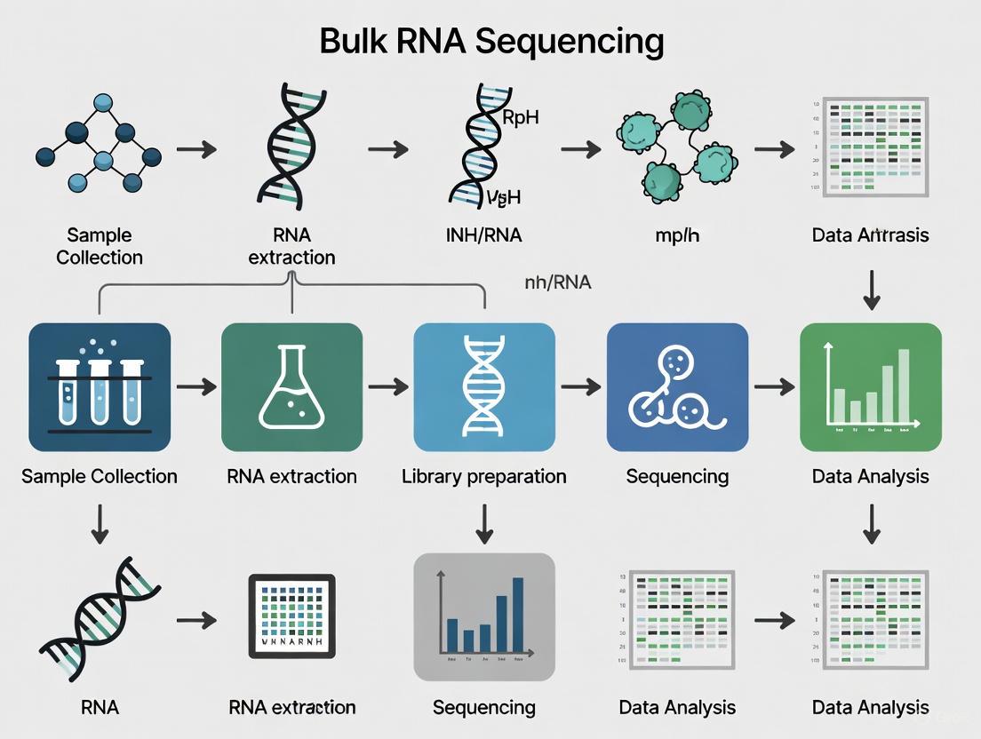
The Bulk RNA-Seq Workflow: A Step-by-Step Guide

The journey from a biological sample to a sequenced library involves a series of critical, interconnected steps. Each stage must be meticulously planned and executed to ensure the generation of high-quality, reliable data. The following diagram provides a high-level overview of the entire process.

Overview of the bulk RNA-seq laboratory workflow

Sample Collection and RNA Extraction

The workflow begins with the collection of biological material, such as tissues, cells, or blood [9]. A critical first step is cell lysis, which involves breaking open cells to release their intracellular contents, including RNA. This is achieved through mechanical methods (e.g., bead beating, homogenization), chemical lysis (using detergents), or enzymatic digestion, often in combination [9].

Following lysis, total RNA isolation is performed. Traditional methods use phenol-chloroform-based reagents like TRIzol or silica column-based purification kits to separate RNA from DNA and proteins [9]. The goal is to obtain high-quality, intact total RNA, which includes messenger RNA (mRNA), ribosomal RNA (rRNA), and various non-coding RNAs. Preserving RNA integrity by minimizing RNase activity is paramount throughout this process [9]. Innovative platforms, such as Singleron's AccuraCode, can streamline this process by using cell barcoding technology to directly label and capture RNAs from lysed cells, eliminating the need for traditional RNA extraction [9].

RNA Quality Control and mRNA Selection

Before proceeding, the quality and quantity of the isolated RNA must be rigorously assessed [9]. RNA Quality Control (QC) typically involves spectrophotometric methods (NanoDrop) or fluorometric assays (Qubit) to measure concentration and purity. More importantly, capillary electrophoresis systems like the Agilent Bioanalyzer provide an RNA Integrity Number (RIN), where a value greater than 7 typically indicates high-quality RNA suitable for sequencing [9]. Poor RNA quality at this stage can lead to biased or unreliable results.

The next step is to enrich for transcripts of interest, most commonly messenger RNA (mRNA). Two primary strategies are employed, each with distinct advantages [9]:

• Poly(A) Selection: This method uses oligo(dT) primers to bind specifically to the polyadenylated tails of mRNAs. It effectively enriches for protein-coding transcripts and is best suited for high-quality RNA samples [9].
• Ribosomal RNA (rRNA) Depletion: This method removes abundant ribosomal RNA species through hybridization-based capture. It is advantageous for analyzing degraded samples (e.g., from FFPE tissues) and for detecting non-polyadenylated transcripts like some long non-coding RNAs (lncRNAs) [9].

Library Preparation and Sequencing

RNA Fragmentation is performed to break the RNA into smaller, manageable fragments of around 200 base pairs, which facilitates efficient downstream sequencing [9]. This can be done enzymatically or chemically.

These RNA fragments are then reverse transcribed into complementary DNA (cDNA) using reverse transcriptase, often with random hexamer or oligo(dT) primers [9]. This step converts the unstable RNA molecules into stable DNA templates.

Finally, cDNA Library Construction involves several steps to make the fragments ready for sequencing [9]:

• End repair and A-tailing: The ends of cDNA fragments are blunted and adenylated.
• Adapter ligation: Short, double-stranded DNA adapters containing platform-specific sequences and sample-specific barcodes (indexes) are ligated to the cDNA fragments.
• PCR amplification: The adapter-ligated cDNA is amplified to increase the material for sequencing.

Protocols like Prime-seq have been developed to enhance cost-efficiency. Prime-seq uses early barcoding and Unique Molecular Identifiers (UMIs) during cDNA generation, allowing samples to be pooled for all subsequent steps, reducing reagent costs and hands-on time [5]. The final prepared libraries are quantified and quality-checked before being loaded onto high-throughput sequencers, such as Illumina's NovaSeq or NextSeq, for sequencing [9].

Key Experimental Considerations and Best Practices

Experimental Design and Replication

A carefully considered experimental design is the most crucial aspect of a successful RNA-seq study [10]. Key considerations include:

• Defining the Hypothesis: The study should begin with a clear hypothesis and aim, which will guide all subsequent decisions, from the model system to the sequencing depth [10].
• Biological Replicates: These are independent biological samples within the same experimental group (e.g., different animals, or cell cultures). They are essential for accounting for natural biological variation and ensuring findings are generalizable [10]. At least 3 biological replicates per condition are typically recommended, though 4-8 is ideal for most experiments to ensure robust statistical power [10].
• Technical Replicates: These involve processing the same biological sample multiple times to assess technical variation introduced by the workflow. While biological replicates are more critical, technical replicates can help monitor technical noise [10].
• Batch Effects: Systematic non-biological variations can arise when samples are processed in different groups or at different times. The experimental layout should be planned to minimize and enable correction for these batch effects during analysis [10].
• Pilot Studies: Running a small-scale pilot study is an excellent way to validate workflows, assess variability, and determine the optimal sample size for the main experiment [10].

Sequencing Depth and Quality Control Standards

Adhering to established sequencing standards is vital for generating publication-quality data. The table below summarizes key quantitative metrics from authoritative sources like the ENCODE consortium.

Table 1: Key Quantitative Standards for Bulk RNA-Seq Experiments

Parameter	Recommended Standard	Notes and Context
Aligned Reads per Replicate	20-30 million	Older projects aimed for 20M; ENCODE standards recommend 30M aligned reads [6].
Replicate Concordance	Spearman correlation >0.9 (isogenic) / >0.8 (anisogenic)	Measure of reproducibility between biological replicates [6].
Read Length	Minimum 50 base pairs	Defined by the ENCODE Uniform Processing Pipeline [6].
Library Insert Size	Average >200 base pairs	Defines a bulk RNA-seq experiment per ENCODE standards [6].
RNA Integrity Number (RIN)	>7	Indicates high-quality, intact RNA suitable for sequencing [9].

The Scientist's Toolkit: Essential Research Reagents

The wet-lab workflow relies on a suite of specific reagents and materials to ensure successful library preparation.

Table 2: Key Research Reagent Solutions in Bulk RNA-Seq

Reagent / Material	Function	Application Notes
TRIzol / Column Kits	For total RNA isolation from lysed cells; separates RNA from DNA and proteins.	Phenol-chloroform-based (TRIzol) or silica-membrane based (kits). Critical for obtaining high-quality input material [9].
DNase I	Enzyme that degrades genomic DNA to prevent contamination in RNA samples.	Essential for accurate quantification, as gDNA can be a source of background noise [5].
Oligo(dT) Beads	For poly(A) selection; binds to polyadenylated tails of mRNAs to enrich for coding transcripts.	Best for high-quality RNA. Removes majority of rRNA and other non-coding RNAs [9].
rRNA Depletion Probes	For ribosomal RNA depletion; uses probes to hybridize and remove abundant rRNA.	Used for degraded samples (FFPE) or to study non-polyadenylated RNAs [9].
Reverse Transcriptase	Enzyme that synthesizes complementary DNA (cDNA) from an RNA template.	High-fidelity enzymes are crucial for preserving transcript diversity and minimizing bias [9].
Platform-Specific Adapters	Short, double-stranded DNA containing sequences for binding to the flow cell and sample barcodes (indexes).	Allows for multiplexing—pooling multiple samples in a single sequencing lane [9].
ERCC Spike-In Controls	Synthetic RNA controls added at known concentrations to the sample.	Serves as an internal standard for assessing technical performance, sensitivity, and quantification accuracy [6] [10].

The bulk RNA-seq workflow is a multi-stage process that transforms biological samples into quantitative gene expression data. Its core components—sample preparation, RNA extraction, quality control, library preparation, and sequencing—must be meticulously executed. Best practices, including robust experimental design with adequate biological replication and adherence to established quality standards, are non-negotiable for generating biologically meaningful and reliable results. As the field advances, the development of more efficient protocols like Prime-seq promises to further increase the accessibility and scalability of this powerful technology [5]. When properly planned and executed, bulk RNA-seq remains an indispensable tool for researchers and drug development professionals exploring the transcriptome.

Within the broader scope of bulk RNA sequencing workflow research, a critical challenge lies in accurately quantifying gene expression from raw sequencing data. This process is inherently statistical, as it must account for two distinct but interconnected levels of uncertainty. The first level involves determining the transcript of origin for each sequenced read, a task complicated by the presence of paralogous genes and alternatively spliced transcripts. The second level concerns the conversion of these often-ambiguous read assignments into a reliable count matrix for downstream differential expression analysis. Effectively managing these uncertainties is fundamental to ensuring that biological interpretations are based on accurate and robust data, a concern of paramount importance for researchers and drug development professionals relying on RNA-seq for biomarker discovery and therapeutic target identification [7] [11].

This technical guide explores the methodologies and computational tools designed to address these challenges, providing a detailed overview of best practices within a modern bulk RNA-seq research framework.

Level 1: Read Assignment Uncertainty

The initial step in RNA-seq analysis involves assigning millions of short sequencing reads to their correct transcripts of origin. This is not a trivial task, as many reads may map equally well to multiple genes or isoforms due to sequence similarity, such as in gene families or regions shared by alternative transcripts [7].

Core Challenges and Solutions

Early bioinformatics approaches often simply discarded multi-mapping reads, leading to significant loss of information and systematic underestimation of gene expression, particularly for genes with low sequence uniqueness [12]. Modern methods have developed sophisticated strategies to handle this ambiguity:

• Probabilistic Assignment: Instead of discarding multi-mapping reads, tools like Salmon and kallisto use probabilistic models to distribute reads across all potential transcripts of origin in proportion to the likelihood of assignment [7]. This pseudo-alignment approach is computationally efficient and avoids the biases introduced by discarding reads.
• Alignment-Based Resolution: An alternative method involves first using splice-aware aligners like STAR to map reads to a genome. The resulting alignments are then processed by tools like RSEM (RNA-Seq by Expectation Maximization), which employs an expectation-maximization algorithm to resolve multi-mapping reads and estimate transcript abundances [7].

The following table summarizes the primary approaches to managing read assignment uncertainty:

Table 1: Computational Strategies for Read Assignment Uncertainty

Method Type	Example Tools	Core Principle	Key Advantage
Pseudo-alignment	Salmon, kallisto [7]	Probabilistic assignment of reads to transcripts without full base-by-base alignment.	Speed and efficiency; direct quantification from FASTQ.
Alignment-Based	STAR (alignment) + RSEM (quantification) [7]	Initial genome/transcriptome alignment followed by statistical resolution of multi-mappers.	Generates alignment files (BAM) useful for quality control and visualization.
Integrated Workflow	nf-core/rnaseq (STAR + Salmon) [7]	Combines alignment for QC with Salmon for accurate quantification.	Provides comprehensive QC metrics alongside high-quality expression estimates.

Level 2: Count Estimation Uncertainty

Once reads are assigned, the next level of uncertainty involves converting these assignments into a final count matrix. This step must account for the confidence (or lack thereof) in the assignments themselves.

Quantifying Inferential Uncertainty

The uncertainty in read assignment propagates to the final expression estimates. Advanced quantification pipelines can now quantify this inferential uncertainty:

• Inferential Replicates: Tools like alevin (for single-cell data) and Salmon can generate "inferential replicates" through bootstrapping or Gibbs sampling. These replicates reflect how quantification estimates might vary due to the randomness of read sampling and ambiguity in assignment [12].
• Compression Techniques: Storing and processing a full set of inferential replicates can be computationally prohibitive. Research shows that storing only the mean and variance of these replicates is sufficient to capture gene-level uncertainty, drastically reducing storage and memory requirements without sacrificing information [12]. These compressed parameters can later be used to generate "pseudo-inferential" replicates for downstream statistical analysis.

Impact on Downstream Analysis

Incorporating quantification uncertainty into differential expression testing has been shown to improve the reliability of results. For example, when statistical frameworks like Swish or tradeSeq are modified to account for this uncertainty, they demonstrate a significant reduction in false positive rates, particularly for genes with high levels of multi-mapping reads [12].

Table 2: Addressing Count Estimation Uncertainty in Downstream Analysis

Concept	Description	Benefit in Downstream Analysis
Inferential Replicates	Multiple estimations of expression from the same sample, representing quantification uncertainty [12].	Provides a measure of confidence for each gene's expression level.
Uncertainty-Aware Differential Expression	Statistical methods (e.g., extended Swish, tradeSeq) that incorporate inferential uncertainty [12].	Reduces false positives by more than a third for genes with high quantification uncertainty [12].
Compression	Storing only the mean and variance of inferential replicates [12].	Reduces disk storage to as low as 9% of original requirements, making uncertainty propagation feasible for large studies [12].

Integrated Experimental and Analytical Workflow

A robust bulk RNA-seq study design integrates solutions for both levels of uncertainty from the start. The following diagram illustrates a recommended workflow that combines experimental best practices with computational methods to manage uncertainty effectively.

Detailed Methodology for an Uncertainty-Aware Workflow

The nf-core/RNA-seq workflow provides a robust, reproducible pipeline that implements best practices for addressing both levels of uncertainty [7].

• Input Data and Preparation:

  • Input: Paired-end FASTQ files from all biological replicates. Paired-end reads are strongly recommended over single-end for more robust expression estimates [7].
  • Genome Reference: A genome FASTA file and a corresponding GTF/GFF annotation file for the organism.

• Core Analysis Steps:

  • Spliced Alignment with STAR: The FASTQ files are aligned to the reference genome using the splice-aware aligner STAR. This step produces BAM files, which are crucial for generating detailed quality control (QC) metrics for each sample [7].
  • Alignment-Based Quantification with Salmon: The genomic alignments from STAR are projected onto the transcriptome and used as input for Salmon running in alignment-based mode. Salmon leverages its statistical model to handle the two levels of uncertainty: it probabilistically resolves read assignment ambiguity (Level 1) and generates accurate transcript-level abundance estimates, often incorporating UMI-based deduplication to improve count estimation (Level 2) [7].
  • Generation of Count Matrices: The nf-core workflow automatically aggregates the sample-level quantification from Salmon into a gene-level count matrix, which is the primary input for differential expression tools like DESeq2 or limma-voom [13] [7].

• Uncertainty Propagation (Optional):

  • For advanced analyses, run Salmon with flags that generate inferential replicates. These can be incorporated into specialized differential expression frameworks like the fishpond package in R to account for quantification uncertainty in statistical testing [12].

The Scientist's Toolkit

Table 3: Essential Research Reagent Solutions and Computational Tools

Item / Tool Name	Function in the Workflow
STAR	Splice-aware aligner for mapping RNA-seq reads to a reference genome; generates alignment files for QC [7].
Salmon	Rapid quantification tool that uses pseudoalignment or alignment to estimate transcript abundance while modeling read assignment uncertainty [7].
nf-core/rnaseq	A comprehensive, community-maintained Nextflow pipeline that automates the entire workflow from FASTQ to count matrix, integrating STAR and Salmon [7].
alevin	A droplet-based scRNA-seq quantification pipeline that extends Salmon's model to single-cell data and can assess quantification uncertainty via bootstrapping [12].
fishpond (R package)	A Bioconductor package containing the Swish method for differential expression analysis that can incorporate inferential replicates to account for quantification uncertainty [12].
DESeq2 / limma	Established R/Bioconductor packages for differential expression analysis of bulk RNA-seq count matrices [13] [7].
Unique Molecular Identifiers (UMIs)	Short random sequences used during library prep to tag individual mRNA molecules, allowing for accurate counting and removal of PCR duplicates [5].

Successfully addressing the dual challenges of read assignment and count estimation uncertainty is not merely a computational exercise but a foundational requirement for generating biologically meaningful results from bulk RNA-seq data. By adopting integrated workflows that leverage probabilistic quantification tools like Salmon, utilizing alignment-based QC, and—for critical applications—propagating inferential uncertainty into statistical testing, researchers can significantly enhance the robustness and reliability of their findings. As the field continues to evolve, with new methods like Prime-seq offering more cost-efficient profiling, the principles of rigorously accounting for technical uncertainty will remain central to advancing transcriptomics research and its applications in drug development and personalized medicine [12] [7] [5].

In the context of broader thesis research on the bulk RNA sequencing workflow, understanding its fundamental trade-offs with single-cell RNA sequencing (scRNA-seq) is paramount for researchers and drug development professionals. The core distinction lies in the resolution trade-off: bulk RNA-seq provides a population-averaged gene expression profile from a tissue or cell population, while scRNA-seq delivers gene expression data at the individual cell level [14] [15]. This difference in resolution creates a cascade of technical and analytical consequences that dictate their appropriate application in research and development pipelines. Bulk RNA sequencing (bulk RNA-seq) is a next-generation sequencing (NGS)-based method that measures the whole transcriptome across a population of thousands to millions of cells, yielding an average expression level for each gene across all cells in the sample [14]. In contrast, single-cell RNA sequencing profiles the whole transcriptome of each individual cell within a sample, enabling the resolution of cellular heterogeneity [14] [15]. This foundational difference drives all subsequent decisions regarding experimental design, cost, computational analysis, and biological interpretation.

Technical Foundations and Workflow Comparisons

Core Methodological Differences

The experimental workflows for bulk and single-cell RNA-seq diverge significantly from the initial sample preparation stage, reflecting their distinct objectives and resolution targets.

• Bulk RNA-seq Workflow: The process begins with RNA extraction directly from the entire biological sample (e.g., tissue, cell culture). The extracted RNA (either total RNA or enriched mRNA) is then converted to cDNA and processed into a sequencing library that represents the pooled genetic material of all cells [14] [16]. This workflow outputs a single expression profile per sample, where each data point represents the average expression level of a gene across the entire cell population.

• Single-Cell RNA-seq Workflow: The initial, critical step involves creating a viable single-cell suspension from the sample through enzymatic or mechanical dissociation [14] [15]. Following quality control to ensure cell viability and absence of clumps, individual cells are partitioned into micro-reaction vessels. In the 10X Genomics platform, this is achieved through a microfluidics system that creates Gel Beads-in-emulsion (GEMs), where each GEM contains a single cell, a gel bead with cell-barcoded oligos, and reverse transcription reagents [14] [15]. Cell lysis occurs within each GEM, allowing captured mRNA to be barcoded with a cell-specific barcode and unique molecular identifier (UMI). This barcoding enables the pooling of all material for sequencing while maintaining the ability to trace transcripts back to their cell of origin during computational analysis [14].

Visualizing Core Workflow Divergence

The following diagram illustrates the fundamental procedural differences between the two sequencing approaches, highlighting the critical branching points that define their respective resolutions.

Quantitative Comparison: Performance Metrics and Applications

The choice between bulk and single-cell RNA-seq involves navigating a complex landscape of technical capabilities, performance trade-offs, and practical constraints. The following table synthesizes key comparative metrics essential for informed experimental design.

Feature	Bulk RNA-Seq	Single-Cell RNA-Seq
Resolution	Population average [14] [17]	Individual cell level [14] [17]
Cost per Sample	Lower (~$300/sample) [17]	Higher (~$500-$2000/sample) [17]
Cell Heterogeneity Detection	Limited; masks differences [14] [17]	High; reveals subpopulations [14] [17]
Rare Cell Type Detection	Not possible; signals diluted [17]	Possible; can identify rare populations [17]
Gene Detection Sensitivity	Higher per sample (detects more genes) [17]	Lower per cell (sparse data, dropouts) [17] [18]
Data Complexity	Lower; simpler analysis [14] [17]	Higher; specialized tools required [14] [17]
Sample Input Requirement	Higher amount of tissue/RNA [17]	Lower; works with few cells [17]
Isoform/Splicing Analysis	More comprehensive [17] [15]	Limited with standard assays [17]
Primary Applications	Differential expression, biomarker discovery, pathway analysis [14] [15]	Cell atlas creation, tumor heterogeneity, rare cell discovery, developmental tracing [14] [17] [15]

Analytical Pipelines and Computational Considerations

Bulk RNA-Seq Data Processing

The computational analysis of bulk RNA-seq data follows a established pathway with robust, standardized tools. The primary goal is to transform raw sequencing reads (FASTQ files) into a gene count matrix for differential expression testing [7] [16].

• Quality Control and Trimming: Initial QC assesses raw read quality using tools like FastQC, followed by trimming of adapters and low-quality bases with tools such as Trimmomatic [16].
• Read Alignment: Quality-controlled reads are aligned to a reference genome using spliced aligners like STAR or TopHat2 that account for exon-intron junctions [7] [16]. Alternatively, pseudoalignment tools like Salmon or kallisto can be used for faster quantification without generating base-level alignments [7].
• Expression Quantification: Aligned reads are assigned to genomic features (genes, transcripts) using count-based tools like featureCounts or HTSeq, or estimation-based methods like RSEM and Salmon [7] [16]. The nf-core/RNAseq workflow provides a comprehensive, standardized pipeline that automates these steps from FASTQ to count matrix [7].
• Differential Expression Analysis: The final count matrix is analyzed in R/Bioconductor using packages like limma, DESeq2, or edgeR to identify genes differentially expressed between conditions [7] [16].

Single-Cell RNA-Seq Data Processing

The analysis of scRNA-seq data is more complex due to its high dimensionality, technical noise, and sparsity. A typical pipeline involves:

• Raw Data Processing and Demultiplexing: Tools like Cell Ranger (10X Genomics) process raw BCL files, perform demultiplexing using the cell barcodes and UMIs, and align reads to generate a feature-barcode matrix [14] [15].
• Quality Control and Filtering: Cells are filtered based on metrics like number of detected genes, total UMI counts, and mitochondrial RNA percentage to remove low-quality cells and doublets [16].
• Normalization and Scaling: Technical variations in sequencing depth are corrected, and counts are scaled to facilitate comparisons between cells.
• Feature Selection and Dimensionality Reduction: Highly variable genes are selected, and dimensionality reduction techniques like PCA are applied.
• Clustering and Visualization: Cells are grouped into clusters based on gene expression similarity using graph-based or k-means algorithms, and visualized in 2D using t-SNE or UMAP [16].
• Cell Type Annotation and Marker Identification: Clusters are annotated to cell types by comparing expression of known marker genes, and differential expression analysis identifies marker genes for each cluster.

The Scientist's Toolkit: Essential Research Reagents and Platforms

Successful execution of transcriptomic studies requires careful selection of reagents, platforms, and analytical tools. The following table catalogues key solutions referenced in the literature.

Category	Item/Reagent	Function in Workflow
Library Prep	Poly-dT Oligos	mRNA enrichment by binding poly-A tail [19]
	rRNA Depletion Kits	Remove ribosomal RNA to enrich for mRNA and other RNA species [19] [15]
	Template Switching Oligos	Used in Smart-seq2 protocol for full-length cDNA amplification [16]
Single-Cell Partitioning	10X Genomics Chromium Controller/X	Microfluidics instrument for partitioning cells into GEMs [14] [15]
	Gel Beads	Contain barcoded oligos (cell barcode, UMI, dT primer) for mRNA capture in GEMs [14] [15]
Sequencing & Analysis	Illumina NGS Platforms	High-throughput sequencing of prepared libraries [14]
	nf-core/RNAseq Pipeline	Standardized Nextflow workflow for bulk RNA-seq analysis (QC, alignment, quantification) [7]
	Cell Ranger Suite	10X Genomics software for demultiplexing, alignment, and counting of scRNA-seq data [14]
Bioinformatics	STAR	Spliced aligner for accurate mapping of RNA-seq reads to genome [7] [16]
	Salmon/Kallisto	Tools for fast transcript-level quantification via pseudoalignment [7]
	Limma/DESeq2/edgeR	R/Bioconductor packages for differential expression analysis of bulk data [7] [16]
	Seurat/Scanpy	Comprehensive toolkits for downstream analysis of scRNA-seq data [16]

Integrated and Emerging Approaches

Hybrid and Complementary Applications

Rather than being mutually exclusive, bulk and single-cell RNA-seq are increasingly used as complementary approaches. A powerful strategy uses scRNA-seq to deconvolve bulk RNA-seq data, inferring cell type-specific (CTS) expression from bulk tissue samples [20]. Methods like EPIC-unmix, bMIND, and CIBERSORTx leverage single-cell reference atlases to estimate both cell type proportions and CTS expression profiles from bulk data, enabling CTS analysis for large cohorts where single-cell profiling is cost-prohibitive [20]. This is particularly valuable for studying diseases like Alzheimer's, where bulk RNA-seq from brain tissue can be deconvolved to identify CTS differentially expressed genes and expression quantitative trait loci (eQTLs) [20].

Beyond Whole Transcriptome: Targeted scRNA-seq

For applications requiring high sensitivity for specific genes, targeted single-cell gene expression profiling provides an alternative to whole transcriptome approaches. By focusing sequencing resources on a predefined panel of genes (dozens to hundreds), targeted methods achieve superior sensitivity, reduce gene dropout, and lower costs per sample [18]. This makes them ideal for validating discoveries from initial whole transcriptome studies, interrogating specific pathways, and developing robust assays for clinical translation in drug development [18].

The choice between bulk and single-cell RNA-seq is not a matter of technological superiority but of strategic alignment with research objectives. Bulk RNA-seq remains the workhorse for hypothesis-driven studies comparing defined conditions, where the goal is to identify population-level transcriptional changes, discover biomarkers, or conduct large-scale cohort studies cost-effectively. Its strengths lie in its robust, standardized workflows, lower cost, and high gene detection sensitivity. Conversely, single-cell RNA-seq is a discovery-oriented tool that excels at unraveling cellular heterogeneity, identifying novel cell types and states, and reconstructing dynamic processes like development and disease progression. Its power comes from its unparalleled resolution, albeit at a higher cost and computational complexity. For researchers and drug development professionals, a pragmatic approach often involves using scRNA-seq for initial discovery and atlas-building, followed by bulk RNA-seq or targeted scRNA-seq for validation and scaling across larger cohorts. Furthermore, computational deconvolution methods now allow for the integration of both data types, maximizing biological insights while navigating practical constraints. Understanding this resolution trade-off is fundamental to designing efficient and informative transcriptomic studies within the broader context of genomic research.

Bulk RNA sequencing (RNA-Seq) is a foundational molecular biology technique that measures the average gene expression profile across a population of cells within a sample [19]. This powerful, large-scale method provides a holistic view of the transcriptome, enabling researchers to make quantitative comparisons between different biological conditions—such as healthy versus diseased tissue or treated versus control samples [19] [14]. By converting RNA molecules into complementary DNA (cDNA) and sequencing them using next-generation sequencing platforms, bulk RNA-Seq captures a global snapshot of transcriptional activity [19]. While newer single-cell technologies resolve cellular heterogeneity, bulk RNA-Seq remains a cornerstone for hypothesis-driven research, particularly in contexts where population-level averages are biologically meaningful or when practical constraints like budget and sample availability prevail [14]. This technical guide explores the primary applications of bulk RNA-Seq, with a focused examination of differential expression analysis and its extensions into broader research domains, framed within the complete workflow of a bulk RNA-Seq study.

The Core Workflow of a Bulk RNA-Seq Experiment

A typical bulk RNA-Seq study follows a multi-stage process, from sample preparation to biological interpretation. The workflow diagram below illustrates the key stages and their interconnections.

From Raw Data to Count Matrix

The initial phase transforms raw sequencing data into a structured gene expression count matrix. This process begins with quality control checks on raw FASTQ files using tools like FastQC, followed by read trimming to remove adapter sequences and low-quality bases [8]. The cleaned reads are then aligned to a reference genome using splice-aware aligners such as STAR [7]. Finally, expression quantification assigns reads to genomic features, generating a count matrix where rows represent genes, columns represent samples, and integer values indicate the number of reads uniquely assigned to each gene [7] [8]. Tools like HTSeq-count or alignment-free tools like Salmon perform this quantification, handling uncertainty in read assignment through statistical models [7].

Key Research Reagent Solutions

The following table details essential reagents and materials required for a successful bulk RNA-Seq experiment.

Table 1: Key Research Reagent Solutions for Bulk RNA-Seq

Item	Function	Examples & Notes
RNA Extraction Kits	Isolate high-quality RNA from source material (cells, tissues).	PicoPure RNA isolation kit [2]. Consider compatibility with sample type (e.g., FFPE, blood).
rRNA Depletion Kits	Remove abundant ribosomal RNA (rRNA) to enrich for mRNA and other RNA types.	Critical for total RNA sequencing. Increases informational yield [19].
Poly(A) Selection Kits	Enrich for messenger RNA (mRNA) by capturing polyadenylated tails.	NEBNext Poly(A) mRNA Magnetic Isolation Module [2]. Standard for mRNA-seq.
Library Prep Kits	Convert RNA into a sequencing-ready library; includes cDNA synthesis, adapter ligation, and indexing.	NEBNext Ultra DNA Library Prep Kit [2]. 3'-Seq kits (e.g., QuantSeq) ideal for high-throughput screens [10].
Spike-in Controls	Add known quantities of exogenous RNA to monitor technical performance and aid normalization.	SIRVs; assess dynamic range, sensitivity, and quantification accuracy [10].
Strandedness Reagents	Preserve the original orientation of RNA transcripts during library construction.	Specified in the library kit (e.g., "forward", "reverse", "unstranded") [7].

Primary Application: Differential Expression Analysis

Differential expression (DE) analysis is the most prominent application of bulk RNA-Seq, statistically identifying genes whose expression levels change significantly between predefined experimental groups [7] [8].

Statistical Foundations and Methodologies

DE analysis operates on the raw count matrix, which typically follows a negative binomial distribution [8]. The core task involves fitting a statistical model to test the null hypothesis that a gene's expression does not differ between conditions (e.g., treated vs. control). Several established tools and packages are available, with DESeq2 and limma being widely adopted for their robustness and accuracy [7] [8].

• DESeq2 employs a negative binomial generalized linear model, internally estimating size factors to account for differences in sequencing depth and dispersion for each gene [8]. It then uses the Wald test or likelihood ratio test to compute p-values for differential expression.
• limma utilizes a linear modeling framework, often with precision weights for count data ("voom" transformation), to assess differential expression [7].

A critical step in DE analysis is multiple testing correction. Due to the simultaneous testing of thousands of genes, the False Discovery Rate (FDR) correction (e.g., Benjamini-Hochberg procedure) is standard to control the expected proportion of false positives among significant results [8]. The outcome is a list of differentially expressed genes (DEGs) with statistics including log2 fold-change, p-value, and adjusted p-value (q-value).

Outputs and Interpretation of DE Analysis

The results of a DE analysis are typically presented in a comprehensive table and visualized to facilitate biological interpretation.

Table 2: Typical Outputs from Differential Expression Analysis (e.g., DESeq2)

Output Column	Description	Biological Interpretation
baseMean	The mean of normalized counts for the gene across all samples.	Provides an estimate of the gene's overall expression level.
log2FoldChange	The log2-transformed ratio of expression between the two groups.	A value of 1 indicates a 2-fold upregulation; -1 indicates a 2-fold downregulation.
lfcSE	The standard error of the log2 fold-change estimate.	Measures the precision of the effect size estimate.
stat	The test statistic (e.g., from the Wald test).	Used to compute the p-value.
pvalue	The nominal p-value from the test of differential expression.	The probability of observing the data if the null hypothesis (no change) is true.
padj	The p-value adjusted for multiple testing (e.g., FDR).	A padj < 0.05 is commonly used to define statistically significant DEGs.
svalue	An optional value indicating confidence in the sign (direction) of the log2FoldChange.	Provides an additional measure of confidence in the result [8].

To illustrate the decision-making process in DE analysis, the following logic flow diagram outlines the key steps from raw data to a validated gene list.

Applications Beyond Differential Expression

While differential expression is a central pillar, the utility of bulk RNA-Seq extends to several other critical areas of research.

Transcriptome Characterization and Isoform Analysis

Bulk RNA-Seq is instrumental in cataloging and characterizing the transcriptome. Unlike microarray technology, it can detect novel transcripts, alternative splicing events, and gene fusions without prior knowledge of the transcriptome [14]. This is particularly valuable for annotating genomes of understudied organisms or for discovering disease-specific isoforms and fusion genes, which can serve as therapeutic targets or biomarkers [14] [21]. Specialized library preparations that preserve strand information are often used for these applications to accurately determine the boundaries and orientations of transcripts.

Pathway and Network Analysis

Moving from individual gene lists to higher-order biological meaning, pathway analysis connects DE results to known biological pathways and gene ontologies [22]. This involves testing for the enrichment of DEGs in predefined gene sets representing metabolic pathways, signaling cascades, or molecular functions. Tools like DAVID and Reactome are commonly used for this purpose, helping researchers interpret their DE findings in the context of cellular processes and systems-level biology [22]. This application is crucial in drug discovery for understanding a compound's mechanism of action and identifying potential on-target and off-target effects [10].

Specialized Applications in Drug Discovery and Development

Bulk RNA-Seq is strategically applied throughout the drug discovery and development pipeline [10]. Its applications in this context include:

• Target Identification: Comparing gene expression profiles of diseased versus healthy tissues to identify dysregulated genes and pathways that can be targeted therapeutically.
• Biomarker Discovery: Identifying RNA-based signatures for patient stratification, diagnosis, prognosis, and monitoring treatment response [14] [10].
• Mode-of-Action Studies: Profiling transcriptomic changes in response to drug treatment to elucidate a compound's biological effects and mechanisms.
• Dose-Response and Combination Studies: Assessing transcriptional changes across different drug doses or combination therapies to determine optimal treatment regimens [10].

Best Practices for Robust Experimental Design

The reliability of any bulk RNA-Seq application hinges on a well-designed experiment. Key considerations to mitigate technical artifacts and false discoveries include:

• Replication: Biological replicates (samples derived from different biological entities) are essential for capturing natural variation and ensuring findings are generalizable. A minimum of three biological replicates per condition is typical, with larger numbers (4-8) recommended for robust statistical power, especially when biological variability is high [10]. Technical replicates (repeated measurements of the same biological sample) are less critical but can help assess technical noise.
• Batch Effects: Systematic non-biological variations introduced when samples are processed in different batches can confound results. Experimental design should randomize samples across processing batches whenever possible. Statistical batch correction methods can be applied during analysis if batch effects are unavoidable [10].
• Controls: Including positive and negative controls strengthens experimental conclusions. Spike-in RNAs (e.g., SIRVs) are valuable external controls for monitoring quantification accuracy and assay performance across samples and batches [10].
• Pilot Studies: For large-scale projects, a pilot study using a representative subset of samples is highly recommended to validate wet-lab and computational workflows before committing significant resources [10].

Bulk RNA-Seq remains an indispensable tool for comprehensive transcriptome profiling. Its primary application in differential expression analysis provides a statistically rigorous framework for identifying genes altered between biological states. However, as this guide illustrates, its utility extends far beyond this core function to encompass transcriptome annotation, pathway analysis, and specialized applications in drug discovery. The successful implementation of a bulk RNA-Seq study—from a hypothesis-driven experimental design and appropriate reagent selection to the application of robust computational pipelines—empowers researchers and drug development professionals to extract profound insights into the molecular underpinnings of health, disease, and therapeutic intervention.

Executing the Bulk RNA-Seq Pipeline: Best Practices from Lab to Analysis

High-quality, intact RNA is a fundamental requirement for successful bulk RNA sequencing, as RNA integrity directly impacts the accuracy and reliability of gene expression data [23]. The susceptibility of RNA to degradation by ubiquitous RNases makes careful handling and proper quality assessment during nucleic acid isolation critical steps in the workflow [23]. Within the broader context of bulk RNA sequencing research, the sample preparation phase serves as the foundation upon which all subsequent analytical steps are built. This technical guide details the methods and considerations for ensuring RNA integrity from initial isolation through quality verification, providing researchers with the knowledge needed to prevent experimental failure and generate robust, reproducible transcriptomic data.

RNA Quality Assessment Methods

A variety of techniques are available to assess RNA concentration, purity, and integrity. Each method offers distinct advantages and limitations, and often they are used in combination to provide a comprehensive quality profile.

Table 1: Methods for RNA Quality Assessment

Method	Principle	Information Provided	Advantages	Disadvantages/Limitations
UV Spectrophotometry (e.g., NanoDrop)	Measures absorbance of ultraviolet light by nucleic acids and contaminants at 260 nm, 280 nm, and 230 nm [23].	Concentration (A260), Purity (A260/A280 and A260/A230 ratios) [23] [24].	Fast (≤30 seconds); small sample volume (0.5–2 µl); wide detection range (2 ng/µl–12,000 ng/µl) [23].	Not sensitive to degradation; lacks specificity between RNA/DNA; overestimation if contaminants absorb at ~260 nm [23] [24].
Fluorometric Assay (e.g., Qubit, QuantiFluor)	Fluorescent dyes bind nucleic acids, undergo conformational change, and emit light [23].	Highly accurate RNA concentration, especially for dilute samples [23] [24].	Extremely sensitive (can detect ≤100 pg/µl); suitable for low-concentration samples [23] [24].	Requires standard curves; dyes may not be RNA-specific (may bind DNA); provides no integrity/purity information [23].
Agarose Gel Electrophoresis	Separates nucleic acid fragments by size using an electric current; visualizes with fluorescent dye [23] [25].	Integrity via sharpness and intensity of ribosomal RNA bands (28S:18S ~2:1 for mammals); can visualize genomic DNA contamination [23] [25].	Relatively low cost; provides visual integrity check [23].	Requires significant RNA (≥200 ng for EtBr); time-consuming; potential safety hazards from stains [23] [25].
Microfluidics Capillary Electrophoresis (e.g., Agilent Bioanalyzer/TapeStation)	Microfluidics and fluorescence dye separate RNA fragments in a chip [23] [25].	RNA Integrity Number (RIN); precise integrity assessment; concentration and purity estimation [2] [25].	High sensitivity (requires only 1 µl of ~10 ng/µl RNA); provides digital integrity score (RIN); fast and automated [25].	Higher instrument cost; not suitable for assessing poly(A)-selected mRNA integrity on gels [25].

Detailed Experimental Protocols for RNA QC

Protocol: UV Spectrophotometry for RNA Purity Assessment

This protocol is used for a rapid initial assessment of RNA sample concentration and purity from contaminants like protein or salts [23] [24].

• Instrument Blanking: Apply 1–2 µl of the elution buffer (e.g., nuclease-free water) used to dissolve the RNA sample to the measurement pedestal. Perform a blank measurement to calibrate the instrument.
• Sample Measurement: Wipe away the blank and apply 1–2 µl of the RNA sample to the pedestal. Measure the absorbance.
• Data Interpretation: Record the concentration and the A260/A280 and A260/A230 ratios. Pure RNA typically has an A260/A280 ratio of 1.9–2.1 and an A260/A230 ratio of >1.7 (often 2.0–2.2) [23] [24]. Significant deviation from these ranges indicates potential contamination that may interfere with downstream applications.

Protocol: Agarose Gel Electrophoresis for RNA Integrity Check

This method provides a visual representation of RNA integrity based on the sharpness of ribosomal RNA bands [25].

• Gel Preparation: Prepare a 1.5% denaturing agarose gel. Denaturing conditions, typically using formaldehyde or glyoxal/DMSO, are essential to prevent RNA secondary structure from affecting migration [25].
• Sample Loading: Mix 200–500 ng of RNA with loading dye. Include an appropriate RNA ladder (size marker) in one lane [25].
• Electrophoresis: Run the gel at a constant voltage (e.g., 5 V/cm) until the dye front has migrated sufficiently.
• Staining and Visualization: Stain the gel with a fluorescent nucleic acid dye such as SYBR Gold or ethidium bromide and visualize under UV light [23] [25].
• Interpretation: Intact total RNA from a eukaryotic sample will display two sharp, clear bands: the 28S rRNA band should be approximately twice as intense as the 18S rRNA band. A smeared appearance, lack of sharp bands, or deviation from the 2:1 ratio indicates degradation [25].

The Scientist's Toolkit: Essential Reagents & Materials

Table 2: Key Research Reagent Solutions for RNA Isolation and QC

Item	Function/Application	Examples/Specifications
Magnetic Nanoparticles	Bind and purify nucleic acids from complex lysates in a scalable, automatable format [26].	Silica-coated iron oxide nanoparticles (e.g., NAxtra); used in KingFisher systems [26].
DNase I, RNase-free	Digests and removes contaminating genomic DNA from RNA preparations, crucial for accurate RNA quantitation and sequencing [23].	Included in many isolation kits or available as a standalone reagent.
Fluorescent Nucleic Acid Dyes	Sensitive detection and quantification of RNA in solution or in gels [23] [25].	Qubit RNA BR/HS Assay Kits (fluorometry); SYBR Gold or SYBR Green II (gel staining, more sensitive than EtBr) [23] [25].
Microfluidics Kits	Integrated chips and reagents for automated RNA quality analysis, providing a RIN [25].	Agilent RNA 6000 Nano/Pico LabChip Kits (for Bioanalyzer) [25].
ERCC Spike-in Controls	Exogenous RNA controls added to samples to provide a standard baseline for normalization and quality monitoring in RNA-seq experiments [1].	Defined mix of synthetic RNAs at known concentrations (e.g., Ambion ERCC Spike-In Mix) [1].
Lysis Buffers	Disrupt cells and inactivate RNases immediately upon sample collection to preserve RNA integrity [26].	Often contain guanidine thiocyanate or other chaotropic salts; component of most commercial kits [23] [26].

Workflow Integration and Decision Pathway

The following diagram illustrates the logical sequence of steps for assessing RNA quality, from initial isolation to final qualification for downstream bulk RNA-seq applications.

The success of a bulk RNA sequencing project is profoundly dependent on the initial steps of sample preparation and nucleic acid isolation. A rigorous, multi-faceted approach to RNA quality control—integrating assessments of concentration, purity, and most critically, integrity—is not merely a preliminary check but a fundamental component of robust experimental design. By adhering to standardized protocols and leveraging the appropriate technologies from the scientist's toolkit, researchers can ensure that their data accurately reflects the biological state under investigation, thereby maximizing the scientific return from costly and time-consuming RNA-seq workflows.

Within the broader context of bulk RNA sequencing workflow research, the initial decision between mRNA and total RNA library construction protocols is a critical foundational choice. Bulk RNA sequencing is a powerful technique that measures the average gene expression level across a population of cells from samples like tissues or biopsies [27]. This method provides a global overview of transcriptomic differences between conditions, such as healthy versus diseased states or treated versus untreated samples [19]. The library construction approach fundamentally shapes all subsequent data generation and interpretation, making this selection a pivotal point in experimental design with significant implications for data quality, research outcomes, and resource allocation.

Understanding the Core Protocols: mRNA-seq vs. Total RNA-seq

The fundamental distinction between mRNA sequencing (mRNA-seq) and total RNA sequencing (Total RNA-seq) lies in which RNA molecules are captured and prepared for sequencing during library construction.

mRNA Sequencing employs a targeted enrichment strategy using poly(A) selection to isolate messenger RNA molecules that contain polyadenylated tails [28] [29]. This method specifically captures protein-coding transcripts while excluding non-coding RNA species. Since mRNAs constitute only 1-5% of total RNA in eukaryotic cells, this approach efficiently focuses sequencing resources on the coding transcriptome [28].

Total RNA Sequencing takes a comprehensive approach by sequencing all RNA molecules after selectively depleting ribosomal RNA (rRNA), which constitutes 80-90% of total cellular RNA [28] [29]. This method captures both coding and non-coding RNAs, including long non-coding RNAs (lncRNAs), microRNAs (miRNAs), transfer RNAs (tRNAs), and other non-coding RNA species [28]. The removal of rRNA allows sequencing resources to be concentrated on the remaining transcriptome.

Table 1: Fundamental Differences Between mRNA-seq and Total RNA-seq Protocols

Feature	mRNA Sequencing	Total RNA Sequencing
Enrichment Method	Poly(A) selection	Ribosomal RNA depletion
RNA Types Captured	Protein-coding polyadenylated mRNAs	Both coding and non-coding RNAs
Transcript Coverage	3'-biased (in 3' mRNA-seq) or full-length	Even coverage across transcript length
rRNA Removal Efficiency	High through positive selection	High through negative depletion

Technical Comparisons and Experimental Considerations

The choice between these protocols significantly impacts multiple aspects of experimental design and data outcomes. Each method offers distinct advantages and limitations that must be weighed against research objectives.

Transcript Coverage and Strandedness differ notably between approaches. Total RNA-seq provides relatively even coverage across the entire transcript length, enabling analysis of splicing patterns, exon-intron boundaries, and transcript isoforms [28] [29]. mRNA-seq methods, particularly 3' mRNA-seq, generate coverage biased toward the 3' end of transcripts [29]. For both methods, strand-specific protocols are available and recommended, as they preserve information about which DNA strand originated the transcript, which is particularly important for distinguishing overlapping genes on opposite strands [28] [30].

Input RNA Requirements and Sample Quality considerations also vary. mRNA-seq generally performs better with limited starting material and is often preferred for low-input applications [28]. However, total RNA-seq may demonstrate superior performance with degraded RNA samples, such as those from Formalin-Fixed Paraffin-Embedded (FFPE) tissues, because it does not rely on intact poly-A tails for capture [29].

Sequencing Depth and Cost Considerations substantially differ between methods. Total RNA-seq typically requires 3 times more sequencing reads than mRNA-seq for equivalent transcriptome coverage due to its broader capture of diverse RNA species [29]. While mRNA-seq generally has lower per-sample sequencing costs, total RNA-seq provides more comprehensive transcriptome information per sample.

Table 2: Performance Characteristics and Practical Considerations

Parameter	mRNA Sequencing	Total RNA Sequencing
Recommended Sequencing Depth	25-50 million reads per sample [28]	100-200 million reads per sample [28]
Ideal Sample Types	High-quality RNA, limited starting material	Various sample types, including degraded RNA
Key Applications	Differential gene expression of coding genes [29]	Whole transcriptome analysis, isoform identification, non-coding RNA study [29]
Cost Efficiency	Lower cost for coding transcript-focused studies	Higher cost but broader information content

Decision Framework: Selecting the Appropriate Protocol

Choosing between mRNA-seq and total RNA-seq requires systematic consideration of multiple experimental factors. The following workflow diagram outlines the key decision points for selecting the optimal protocol:

This decision pathway emphasizes how research questions should drive technical selections, with practical constraints influencing the final choice.

The Scientist's Toolkit: Essential Research Reagents

Successful library construction requires specific reagents and materials tailored to each protocol. The following table details essential components for both approaches:

Table 3: Essential Reagents for RNA-seq Library Construction

Reagent/Material	Function	Protocol Application
Oligo-dT Magnetic Beads	Binds to poly-A tails for mRNA enrichment	mRNA-seq
rRNA Depletion Probes	Hybridizes to ribosomal RNA for removal	Total RNA-seq
Reverse Transcriptase	Synthesizes cDNA from RNA templates	Both
Random Hexamer Primers	Primes cDNA synthesis across entire transcriptome	Total RNA-seq
Strand-Specific Adapters	Preserves strand orientation information during sequencing	Both
Fragmentation Enzymes	Fragments RNA or cDNA to optimal sequencing size	Both (method varies)
Library Amplification	Amplifies final library for sequencing	Both
Quality Control Assays	Assesses RNA integrity and library quality (e.g., Bioanalyzer, Qubit) [27]	Both

Experimental Workflow: From Sample to Sequence

Both mRNA-seq and total RNA-seq share common procedural phases but differ significantly in key steps. The following diagram illustrates the complete workflow with critical divergence points:

The critical divergence occurs during library construction, where either poly-A selection (mRNA-seq) or rRNA depletion (Total RNA-seq) is applied. Subsequent steps of cDNA synthesis, adapter ligation, and library preparation follow similar pathways, though with potential protocol-specific variations in enzymes and reaction conditions.

The selection between mRNA and total RNA protocols for bulk RNA sequencing library construction represents a fundamental strategic decision with far-reaching implications for research outcomes. mRNA-seq provides a cost-effective, focused approach for differential expression analysis of protein-coding genes, while total RNA-seq offers comprehensive transcriptome coverage at higher complexity and cost. There is no universally superior option—the optimal choice emerges from careful alignment of technical capabilities with specific research questions, sample characteristics, and resource constraints. By applying the systematic decision framework presented herein, researchers can make informed choices that maximize the scientific return on their investment in transcriptomic studies, ensuring that library construction protocols effectively support their overarching research objectives within the broader context of bulk RNA sequencing workflows.

The selection of an appropriate next-generation sequencing (NGS) platform and the determination of optimal sequencing depth are fundamental decisions in bulk RNA sequencing workflow research. These choices directly impact data quality, experimental outcomes, and resource allocation, particularly in drug discovery and development contexts. With continuous innovation driving down costs, NGS has become increasingly accessible to laboratories of all sizes, enabling researchers to expand the scale and discovery power of their genomics studies [31]. The cost of sequencing has seen a dramatic 96% decrease in the average cost-per-genome since 2013, making the technology more affordable than ever [31]. However, researchers must adopt a holistic view when evaluating NGS costs, considering not just the instrument price or cost per gigabase, but the total cost of ownership, which includes setup, ancillary equipment, ease of use, support, training, and data analysis capabilities [31].

For bulk RNA-seq experiments in drug discovery, careful experimental design is the most crucial aspect for ensuring meaningful results [10]. The balance between cost and data quality requires thoughtful consideration of multiple factors, including research goals, sample availability, biological variability, and the specific questions being addressed. This technical guide provides comprehensive recommendations for selecting sequencing platforms, determining appropriate depth requirements, and implementing cost-effective strategies for bulk RNA sequencing workflows within the context of pharmaceutical and basic research applications.

Sequencing Platform Comparison and Selection

Platform Specifications and Performance Metrics

When selecting a sequencing platform for bulk RNA-seq, researchers must evaluate key performance parameters across available systems. The specifications of two representative high-throughput platforms are compared in the table below:

Table 1: Comparison of High-Throughput Sequencing Platforms

Parameter	Illumina NovaSeq 6000	DNBSEQ-T7
Maximum Output	6 Tb (S4 flow cell)	7 Tb (4 flow cells)
Read Lengths	50-300 bp paired-end	100-150 bp paired-end
Reads per Flow Cell	Up to 10 billion (S4)	Up to 5.8 billion (4 FC)
Run Time (PE150)	Approximately 44 hours	22-24 hours
Q30 Score	>85% (typical)	>85%
Key Technology	Sequencing by synthesis	DNA nanoball sequencing

Data compiled from manufacturer specifications [32] and industry standards [31].

The DNBSEQ-T7 platform exemplifies recent advancements, offering flexible run configurations with four independent flow cells, enabling researchers to process multiple projects simultaneously with varying scale requirements [32]. This platform demonstrates low GC bias and consistent data quality across diverse sample types, making it suitable for various RNA-seq applications in clinical research, population studies, and microbiology [32]. Similarly, Illumina platforms continue to evolve with innovations focused on operational simplicity and streamlined workflows, benefiting from a comprehensive ecosystem of supported applications and analysis tools [31].

Cost Considerations Beyond Instrument Price

The initial instrument cost represents only one component of the total investment required for successful NGS implementation. A comprehensive assessment must include:

• Running expenses: Cost per experiment including DNA/RNA isolation, library preparation, and sequencing reagents [31]
• Laboratory infrastructure: Nucleic acid quantitation instruments, quality analyzers, thermocyclers, centrifuges, and other ancillary equipment [31]
• Data management: Storage solutions, server maintenance, software licenses, and computational resources for analysis [31]
• Personnel costs: Training requirements, hands-on time, and technical expertise needed for operation and troubleshooting [31]

Economies of scale can significantly reduce costs for higher-output applications, with multiplex sequencing enabling exponential increases in sample throughput without proportional cost increases [31]. Researchers should also investigate equipment trade-in programs, leasing options, and reagent bundles to optimize financial outlay [31].

Sequencing Depth Recommendations for Bulk RNA-Seq

Coverage Guidelines by Application

Sequencing depth requirements vary significantly across different NGS applications. The following table summarizes recommended coverage levels for common genomic analyses:

Table 2: Sequencing Coverage Recommendations by Method

Sequencing Method	Recommended Coverage	Key Considerations
Whole Genome Sequencing (WGS)	30× to 50× for human	Dependent on application and statistical model
Whole-Exome Sequencing	100×	Standard for variant calling
Bulk RNA Sequencing	10-50 million reads per sample	Dependent on gene expression levels and experimental goals
ChIP-Seq	100×	Standard for transcription factor binding studies

Based on Illumina recommendations [33] and community standards.

For bulk RNA sequencing, depth requirements are typically calculated in terms of the number of millions of reads to be sampled rather than traditional coverage metrics [33]. The detection of rarely expressed genes often requires increased sequencing depth, while more abundant transcripts can be reliably quantified with lower read counts [34]. In human cells, approximately 80% of transcripts expressed at >10 fragments per kilobase of exon per million reads mapped (FPKM) can be accurately quantified with around 36 million 100-bp paired-end reads [34].

Calculating and Achieving Desired Coverage

The Lander/Waterman equation provides a theoretical method for computing genome coverage: C = LN/G, where C represents coverage, G is the haploid genome length, L is the read length, and N is the number of reads [33]. This equation helps researchers estimate the reagents and sequencing runs needed to achieve their desired sequencing coverage [33].

Researchers may need to increase coverage beyond initial estimates for several reasons:

• Adding statistical power to the assay, particularly for detecting subtle expression changes
• Investigating very rare biological events or low-abundance transcripts
• Meeting minimum coverage thresholds required by journals or specific fields
• Sequencing challenging genomic regions or working with complex genomes [33]

Increased coverage can be achieved by combining sequencing output from multiple flow cells or sequencing runs, though this approach increases both cost and computational requirements.

Experimental Design for Optimal Depth and Quality

Sample Size and Replication Strategies

A carefully considered experimental design is paramount for generating statistically robust RNA-seq data. The sample size for a drug discovery project significantly impacts the quality and reliability of the results, with statistical power referring to the ability to identify genuine differential gene expression in naturally variable datasets [10]. Several factors influence sample size decisions, including biological variation, study complexity, cost constraints, and sample availability [10].

Replication strategy is equally critical for accounting for variability within and between experimental conditions:

• Biological replicates: Independent samples for the same experimental group or condition that account for natural variation between individuals, tissues, or cell populations. At least three biological replicates per condition are typically recommended, with 4-8 replicates per sample group covering most experimental requirements [10].
• Technical replicates: The same biological sample measured multiple times to assess technical variation introduced during library preparation or sequencing. While useful for quality control, biological replicates are generally more critical for drawing meaningful biological conclusions [10].

Consulting with bioinformaticians or data experts during the experimental design phase is highly valuable for optimizing study design and ensuring appropriate statistical power [10]. Pilot studies represent an excellent approach for determining optimal sample size by assessing preliminary data on variability and testing various conditions before committing to large-scale experiments [10].

RNA-Seq Specific Design Considerations

Bulk RNA-seq experimental design requires special attention to several key aspects:

• Library preparation: The choice between 3'-end sequencing (e.g., QuantSeq) for gene expression analysis and whole transcriptome approaches for isoform detection depends on the research questions [10]. For large-scale drug screens based on cultured cells, 3'-seq approaches with library preparation directly from lysates can save time and money by omitting RNA extraction [10].
• Batch effects: Systematic, non-biological variations can arise from how samples are collected and processed. Experimental designs should minimize batch effects through randomization and include appropriate controls to enable computational correction during analysis [10].
• Spike-in controls: Artificial RNA controls, such as SIRVs, are valuable tools for measuring assay performance, especially dynamic range, sensitivity, reproducibility, and quantification accuracy [10].
• Strandedness: Library construction protocol determines whether strand information is preserved, which is particularly important for distinguishing overlapping transcripts on opposite strands.

Bulk RNA-Seq Data Analysis Workflow

From Raw Data to Expression Quantification

The bulk RNA-seq analysis workflow involves multiple steps to convert raw sequencing data into biologically interpretable results. The following diagram illustrates the core workflow:

Bulk RNA-seq Analysis Pipeline

Current best practices for expression quantification involve addressing two levels of uncertainty: (1) identifying the most likely transcript of origin for each RNA-seq read, and (2) converting read assignments to a count matrix while modeling assignment uncertainty [7]. Two primary approaches have emerged:

• Alignment-based approaches: Formal alignment of sequencing reads to a genome or transcriptome using splice-aware aligners like STAR, producing BAM files that record exact coordinates of sequence matches [7].
• Pseudoalignment approaches: Faster methods that use substring matching to probabilistically determine locus of origin without base-level precision, implemented in tools like Salmon and kallisto [7].

A hybrid approach is often recommended, using STAR to align reads to the genome for quality control metrics, then using Salmon in alignment-based mode to perform expression quantification that handles uncertainty in converting read origins to counts [7]. This approach leverages the strengths of both methods while providing comprehensive quality assessment.

Differential Expression and Downstream Analysis

Once count data is generated, statistical analysis identifies genes showing different expression levels between conditions. The limma package provides a robust framework for differential expression analysis built on a linear modeling approach [7]. This method offers flexibility in experimental design and has been shown to perform well with bulk RNA-seq data.

Automated tools like Searchlight can significantly reduce the time and effort required for data exploration, visualization, and interpretation (EVI) [35]. Searchlight provides comprehensive statistical and visual analysis at global, pathway, and single-gene levels through three complementary workflows:

• Normalized Expression (NE) workflow: Explores expression data with PCA, sample distance analysis, and highly expressed gene identification [35].
• Differential Expression (DE) workflow: Visualizes single comparisons between two conditions with MA plots, volcano plots, significant gene heatmaps, and pathway analysis [35].
• Multiple Differential Expression (MDE) workflow: Explores relationships between two or more sets of differential comparisons with overlap analysis and signature profiling [35].

These automated pipelines can complete bulk RNA-seq projects to manuscript quality in significantly less time than manual R-based analyses while maintaining flexibility through customizable R scripts [35].

The Scientist's Toolkit: Essential Research Reagents and Materials

Successful bulk RNA-seq experiments require specific reagents and materials throughout the workflow. The following table details essential components:

Table 3: Essential Research Reagents and Materials for Bulk RNA-Seq

Category	Item	Function
Sample Preparation	RNA isolation kits	Extract high-quality RNA from various sample types
	DNase I treatment	Remove genomic DNA contamination
	RNA integrity analyzer	Assess RNA quality (RIN score)
Library Preparation	Poly(A) selection beads	mRNA enrichment from total RNA
	Ribosomal depletion kits	Remove abundant ribosomal RNA
	Reverse transcriptase	Synthesize cDNA from RNA templates
	Second-strand synthesis	Create double-stranded cDNA
	Library adapters	Add platform-specific sequences for clustering
	Unique molecular identifiers (UMIs)	Correct for PCR amplification bias
Sequencing & QC	Quantitation instruments	Precisely measure nucleic acid concentration
	Size selection beads	Remove adapter dimers and select insert size
	Sequencing reagents	Platform-specific chemistry for base calling
	PhiX control	Add sequencing process control
Data Analysis	Reference genomes	Sequence alignment and mapping
	Annotation files (GTF/GFF)	Gene model information for quantification
	Spike-in controls (SIRVs)	Normalization and technical variation assessment

Based on experimental guidelines [10] [7] and manufacturer recommendations.

The selection of appropriate library preparation methods depends on sample type, data requirements, sample numbers, input amounts, and cost considerations [10]. For gene expression and pathway analysis, 3' mRNA-seq methods (e.g., QuantSeq) provide cost and time efficiencies, particularly for large sample numbers through pooled library preparation approaches [10]. When working with challenging sample types like whole blood or FFPE material, specialized workflows and extraction methods are necessary to address issues related to contaminants, abundant transcripts, and degraded RNA [10].

Selecting appropriate sequencing platforms and determining optimal depth requirements for bulk RNA-seq requires careful consideration of multiple competing factors. There is no universal solution that applies to all experimental scenarios—the optimal balance between cost and data quality must be determined based on specific research questions, sample characteristics, and analytical requirements. As sequencing technologies continue to evolve, with both established and emerging platforms offering improved throughput, accuracy, and efficiency, researchers have an expanding array of options to support their scientific investigations.

By applying the principles outlined in this technical guide—understanding platform capabilities, following depth recommendations, implementing robust experimental designs, and utilizing appropriate analysis workflows—researchers can make informed decisions that maximize the scientific return on investment while maintaining high data quality standards. This strategic approach to balancing cost and quality considerations ensures that bulk RNA-seq experiments generate reliable, reproducible, and biologically meaningful results that advance understanding of gene expression regulation in health and disease.

Bulk RNA Sequencing (Bulk RNA-Seq) is a powerful method for transcriptomic analysis of pooled cell populations or tissue sections, providing a quantitative profile of the average gene expression across hundreds to millions of input cells [27]. The bioinformatics processing of this data transforms raw sequencing reads into biologically meaningful information, primarily through two core computational pillars: alignment (determining the genomic origin of reads) and quantification (estimating expression levels) [7]. This processing is a critical component of a broader bulk RNA sequencing workflow, enabling researchers to identify transcriptomic changes associated with disease states, therapeutic responses, and other experimental conditions [30].

The complexity of RNA-Seq data demands a structured bioinformatics approach to account for technical challenges such as reads that map to multiple genes or isoforms, variable sequencing depth, and library preparation artifacts [36]. Proper statistical handling of these challenges is essential for generating accurate, interpretable results that can reliably inform downstream biological conclusions and drug development decisions [2].

Read Alignment & Preprocessing

Alignment Tools and Strategies

The first major step after obtaining raw sequencing reads (FASTQ files) is aligning them to a reference genome or transcriptome. This process determines the transcript of origin for each read and is complicated by the need for "splice-awareness" to handle reads spanning exon-intron boundaries [7].

Table 1: Common Alignment Tools for Bulk RNA-Seq

Tool	Primary Method	Key Features	Considerations
STAR [37] [38]	Splice-aware genome alignment	Fast mapping speed, handles splice junctions directly	Memory intensive
HISAT2 [37]	Memory-efficient genome alignment	Uses fewer memory resources than STAR	Suitable for environments with limited RAM
Bowtie2 [36]	Transcriptome alignment	Often used within RSEM pipeline for transcript quantification	Requires transcript sequences as reference
Salmon [7] [37]	Pseudo-alignment	Extremely fast, avoids full base-by-base alignment	Does not produce base-level alignment files for visualization

Two principal alignment strategies exist. The alignment-based approach (e.g., using STAR or HISAT2) involves formal base-by-base alignment to a reference genome, producing SAM/BAM files that record exact match coordinates. This method is computationally intensive but generates valuable data for quality checks and visualization. The pseudo-alignment approach (e.g., using Salmon or kallisto) uses rapid substring matching to probabilistically determine a read's origin without precise base-level alignment, offering significant speed advantages, particularly for large datasets [7].

For comprehensive analysis, a hybrid approach is often recommended. This involves using STAR to align reads to the genome (facilitating quality control metrics) and then using Salmon in an alignment-based mode to perform quantification from the generated BAM files, leveraging its statistical model for handling assignment uncertainty [7].

Preprocessing and Quality Control

Before alignment, raw sequencing data must undergo quality control and preprocessing to ensure reliable results. The standard workflow includes:

• Quality Assessment: Tools like FastQC provide initial quality metrics on raw reads, including per-base sequence quality, adapter content, and GC content [37] [38].
• Adapter Trimming and Quality Trimming: Trimmomatic or Trim Galore! are used to remove adapter sequences and trim low-quality bases from read ends. This step is crucial for improving mapping rates and downstream analysis accuracy [37] [38].
• Ribosomal RNA Removal (Optional): SortMeRNA can be used to identify and remove reads originating from ribosomal RNA, thereby increasing the proportion of informative mRNA reads [37].

After alignment, tools like RSeQC, Qualimap, and MultiQC aggregate key metrics such as the percentage of uniquely mapped reads, ribosomal RNA content, and coverage uniformity. A uniquely mapped reads percentage of >60-70% is generally considered acceptable [37] [38].

Expression Quantification

Quantification Tools and Outputs

Quantification converts alignment data into numerical estimates of gene or transcript abundance. This step must statistically handle the uncertainty inherent in assigning reads that map to multiple genes or isoforms [7] [36].

Table 2: Quantification Tools and Their Key Outputs

Tool	Quantification Level	Core Outputs	Key Statistical Approach
Salmon [7] [37]	Transcript-level	Estimated counts, TPM (Transcripts Per Million)	Pseudo-alignment or alignment-based modeling with EM algorithm
RSEM [37] [36]	Gene & Isoform-level	Expected counts, TPM, FPKM	Expectation-Maximization (EM) algorithm to resolve multi-mapping reads
featureCounts [37] [38]	Gene-level	Raw read counts	Assigns reads to genomic features (e.g., genes) based on overlap

The two primary levels of quantification are:

• Gene-level quantification provides a collective measure of expression for all transcripts from a single gene locus. Tools like featureCounts and the gene-level summaries from RSEM or Salmon (coupled with transcript-to-gene mapping) generate this data, which is often sufficient for differential gene expression analysis [37] [39].
• Transcript-level (Isoform-level) quantification estimates the abundance of individual splice variants within a gene. This is more computationally challenging due to the high sequence similarity between isoforms of the same gene. Salmon and RSEM are specifically designed for this task and use statistical models (e.g., Expectation-Maximization) to probabilistically resolve the origin of ambiguously-mapping reads [7] [36].

The final output of quantification is a count matrix, where rows correspond to genes/transcripts, columns correspond to samples, and values represent the estimated abundance. This matrix is the fundamental input for downstream differential expression analysis [7].

Integrated Analysis Pipeworks

To enhance reproducibility and efficiency, integrated workflows like the nf-core/rnaseq pipeline automate the entire process from raw FASTQ files to count matrices. This Nextflow-based workflow can seamlessly chain together trimming, alignment (with STAR, HISAT2, or Salmon), quantification (with Salmon or RSEM), and comprehensive quality control, ensuring a standardized and portable analysis [7] [37].

Key Outputs and Data Interpretation

Primary Quantification Outputs

The quantification process generates several key data files that serve different purposes in downstream analysis and interpretation.

• Raw Counts Matrix: This table contains the estimated number of reads assigned to each gene or transcript per sample. These values are not normalized for technical factors like sequencing depth and are the required input for differential expression tools like DESeq2 and limma, which perform their own internal normalization [8] [39].
• Normalized Abundance Estimates: Tools like Salmon and RSEM also output normalized values such as TPM (Transcripts Per Million) and FPKM (Fragments Per Kilobase of transcript per Million mapped reads). These metrics are useful for comparing expression levels of different genes within a sample or for visualizing expression patterns, as they account for both gene length and sequencing depth [37] [36].

Quality Control and Diagnostic Outputs

Beyond the count data, the bioinformatics pipeline produces numerous QC outputs essential for validating data integrity.

• Alignment Statistics: Reports from aligners like STAR detail metrics such as the percentage of uniquely mapped reads, multi-mapped reads, and unmapped reads, which are aggregated by MultiQC [37].
• Pseudoalignment and Quantification Diagnostics: Salmon and RSEM generate logs and auxiliary files that can include 95% credibility intervals for abundance estimates and model fit information [36].
• Sample Similarity Metrics: Prior to differential expression testing, exploratory analyses like Principal Component Analysis (PCA) are performed on the normalized count matrix. PCA plots visualize the largest sources of variation in the dataset and help assess sample grouping, identify potential outliers, and detect batch effects [8] [39] [2].

Workflow Visualization

The following diagram illustrates the logical flow and key decision points in a standard bulk RNA-seq bioinformatics processing workflow.

Figure 1: Bulk RNA-seq Bioinformatics Processing Workflow. This diagram outlines the key steps from raw data to a count matrix, highlighting major alignment and quantification strategies.

The Scientist's Toolkit

Table 3: Essential Research Reagent Solutions for Bulk RNA-Seq Analysis

Category	Item / Tool	Function / Purpose
Reference Files	Genome FASTA File	The reference genome sequence for read alignment [7] [8].
	Annotation File (GTF/GFF)	Contains genomic coordinates of genes, transcripts, and exons, used for alignment and read counting [7] [38].
Software & Pipelines	nf-core/rnaseq	A portable, reproducible Nextflow pipeline automating the entire workflow from FASTQ to counts and QC [7] [37].
	DESeq2 / limma	R/Bioconductor packages for statistical testing of differential expression from count matrices [7] [8].
QC & Visualization	FastQC / MultiQC	FastQC performs initial quality checks on raw reads; MultiQC aggregates results from multiple tools into a single report [37] [38].
	RSeQC / Qualimap	Provide a suite of metrics to evaluate RNA-seq specific data quality post-alignment [37].

Bulk RNA sequencing (RNA-seq) measures the average gene expression levels from complex tissues comprising multiple cell types. While this technology has been instrumental in identifying population-level expression changes, it obscures the transcriptional contributions of individual cell types, limiting insights into cellular heterogeneity. Computational deconvolution has emerged as a powerful set of methodologies to address this limitation by inferring cell-type-specific (CTS) expression and composition from bulk RNA-seq data [40] [41]. These approaches leverage single-cell or single-nuclei RNA sequencing (sc/snRNA-seq) references to dissect bulk expression profiles, enabling researchers to uncover cellular heterogeneity without the substantial costs and technical challenges associated with profiling large sample cohorts at single-cell resolution [42]. The integration of deconvolution into the bulk RNA-seq workflow represents a paradigm shift, allowing researchers to extract cellular-level information from existing and new bulk datasets, thereby bridging the gap between traditional bulk profiling and high-resolution single-cell technologies [40] [43].

The fundamental principle underlying deconvolution is that bulk gene expression represents a weighted average of expression from all constituent cell types, where the weights correspond to cell-type proportions [44]. This relationship can be modeled as B = C × P, where B is the bulk expression matrix, C is the cell-type-specific expression signature matrix, and P is the proportion matrix of cell types across samples. While early deconvolution methods focused primarily on estimating cell-type proportions [41], newer "aggressive" methods aim to reconstruct sample-specific CTS expression profiles, effectively generating k sample-by-gene matrices (where k is the number of cell types) from a single bulk expression matrix [40]. This capability is particularly valuable for identifying cell-type-specific differential expression, expression quantitative trait loci (eQTLs), and other functional genomic elements that would otherwise be masked in bulk analyses [40].

Core Methodologies and Algorithmic Approaches

Taxonomy of Deconvolution Methods

Computational deconvolution methods can be broadly categorized into two classes based on their objectives and outputs. Traditional deconvolution methods focus primarily on estimating cell-type proportions or fractions within bulk samples. This category includes established tools such as CIBERSORT, MuSiC, and Bisque [40] [41]. These methods typically use regression-based frameworks to decompose bulk expression into constituent cell-type proportions using reference signatures derived from purified cell populations or sc/snRNA-seq data [44] [41]. In contrast, aggressive deconvolution methods aim to reconstruct complete sample-level CTS expression profiles, generating separate expression matrices for each cell type present in the bulk mixture. This category includes tools such as TCA, CIBERSORTx, bMIND, BayesPrism, and the recently developed EPIC-unmix [40]. These more ambitious approaches model bulk expression as the weighted sum of CTS expression, using various statistical and computational techniques to solve this ill-posed inverse problem.

Table 1: Categories of Computational Deconvolution Methods

Method Category	Representative Tools	Primary Output	Key Applications
Traditional Methods	CIBERSORT, MuSiC, Bisque, SQUID	Cell-type proportions/fractions	Composition analysis, association studies with phenotypes
Aggressive Methods	TCA, CIBERSORTx, bMIND, BayesPrism, EPIC-unmix	Sample-level CTS expression profiles	CTS differential expression, CTS eQTL mapping, functional genomics

Mathematical Frameworks and Algorithms

Deconvolution methods employ diverse mathematical frameworks to address the computational challenge of inferring cell-type-specific information from bulk data. Regression-based approaches form a foundational category, with methods like MuSiC employing weighted non-negative least squares (W-NNLS) regression that leverages all shared genes between bulk and single-cell data, weighting each gene by cross-subject and cross-cell variations [44]. Bisque implements a similar NNLS framework but incorporates gene-specific transformations of bulk expression to account for technical biases between sequencing technologies [41]. Bayesian methods represent another important category, with tools like bMIND and EPIC-unmix employing empirical Bayesian frameworks to integrate sc/snRNA-seq reference data with bulk RNA-seq data. EPIC-unmix specifically uses a two-step empirical Bayesian approach that first infers CTS expression using a framework similar to bMIND, then adds another layer of Bayesian inference based on priors derived from target samples, making the model data-adaptive to differences between reference and target datasets [40]. Machine learning approaches include methods like CIBERSORTx, which uses support vector regression (SVR), and SQUID, which combines RNA-seq transformation with dampened weighted least-squares deconvolution [42].

Fig. 1: Overview of computational deconvolution workflows. Methods utilize bulk RNA-seq data and single-cell references to estimate either cell type proportions or full expression profiles.

Performance Evaluation and Benchmarking Insights

Comparative Performance Across Methods

Systematic evaluations of deconvolution methods have revealed important differences in accuracy, robustness, and computational efficiency. In comprehensive simulations using the ROSMAP human brain dataset, EPIC-unmix demonstrated superior performance, achieving up to 187.0% higher median Pearson Correlation Coefficient (PCC) and 57.1% lower median Mean Squared Error (MSE) across cell types compared to competing methods including TCA, bMIND, CIBERSORTx, and BayesPrism [40]. The same study also highlighted EPIC-unmix's robustness to the choice of reference panels, showing less loss in prediction accuracy compared to bMIND when using external references from PsychENCODE versus matched internal references [40]. Bisque has shown notable performance advantages in scenarios with significant technical variation between reference and bulk expression technologies, maintaining robust accuracy (R ≈ 0.85, RMSD ≈ 0.07) even at high levels of simulated bias, while other methods like MuSiC, BSEQ-sc, and CIBERSORT showed substantially degraded performance (R ≈ -0.11, RMSD ≈ 0.43) under similar conditions [41].

The SCDC method introduces a unique ENSEMBLE approach that integrates deconvolution results from multiple scRNA-seq reference datasets, implicitly addressing batch effects by assigning higher weights to references that better recapitulate the true underlying bulk expression profiles [44]. This approach has demonstrated improved accuracy over methods using single references, particularly in complex tissues with substantial biological and technical variability. SQUID has also shown promising performance in predicting composition of cell mixtures and tissue samples, with analyses suggesting that it was the only method whose subclone-abundance estimates were predictive of outcomes in RNA-seq-profiled pediatric acute myeloid leukemia and neuroblastoma diagnostic samples [42].

Table 2: Performance Comparison of Selected Deconvolution Methods

Method	Algorithmic Approach	Key Strengths	Reported Performance Metrics
EPIC-unmix	Two-step empirical Bayesian	Robust to reference-target differences; excellent CTS expression inference	187% higher median PCC than competitors; minimal accuracy loss with external references [40]
Bisque	Non-negative least squares with gene-specific transformations	Robust to technical biases; efficient computation	R = 0.923, RMSD = 0.074 in adipose tissue; maintains performance with technological differences [41]
SCDC	ENSEMBLE integration of multiple references	Reduces batch effects; leverages multiple datasets	Improved accuracy over single-reference methods; better phenotype associations [44]
SQUID	RNA-seq transformation + dampened WLS	Optimized for concurrent RNA-seq and scnRNA-seq profiles	Predictive of clinical outcomes in cancer datasets [42]
CIBERSORTx	Support vector regression/machine learning	Batch correction mode; well-established	Outperformed by Bisque in bias scenarios (R = 0.687 vs 0.923) [41]

Impact of Gene Selection and Data Processing

A critical factor influencing deconvolution accuracy is the selection of appropriate genes for analysis. Research has demonstrated that employing a strategic gene selection strategy based on cell-type marker genes and agreement among sc/snRNA-seq datasets and CTS bulk RNA-seq data can significantly enhance performance. In the EPIC-unmix evaluation, selected genes demonstrated 45.2% higher mean PCC and 56.9% higher median PCC compared to unselected genes across all cell types [40]. This advantage was consistent across different reference panels and deconvolution methods, indicating the robustness of a careful gene selection strategy. The optimal gene set for brain tissue analysis included 1,003, 1,916, 764, and 548 genes for microglia, excitatory neurons, astrocytes, and oligodendrocytes, respectively [40].

Data normalization and transformation also significantly impact deconvolution outcomes. Studies have revealed that the distinct nature of technologies used to generate bulk and single-cell sequencing data can introduce gene-specific biases that violate the direct proportionality assumptions of regression-based methods [41]. For example, comparisons between snRNA-seq and bulk RNA-seq data in adipose tissue showed best-fit lines with a mean slope of roughly 0.30 and substantial variance (5.67), indicating significant and variable biases between technologies [41]. Methods that explicitly account for these technical variations, such as Bisque's gene-specific transformations and CIBERSORTx's batch correction mode, generally achieve improved performance compared to methods assuming direct proportionality.

Experimental Protocols and Implementation Guidelines

Reference-Based Deconvolution Workflow

A robust deconvolution analysis requires careful execution of multiple sequential steps. The following protocol outlines a comprehensive workflow for reference-based deconvolution, adaptable to various biological contexts and research questions:

• Reference Data Curation and Preprocessing: Obtain sc/snRNA-seq data from relevant tissues and process using standard pipelines (e.g., Seurat, Scanpy). Essential preprocessing steps include quality control to remove low-quality cells and empty droplets, normalization, batch effect correction, and cell-type annotation using established marker genes [4]. For the reference data, remove cells with abnormally high mitochondrial gene expression (indicating apoptosis or broken membranes) and those with unexpectedly high counts (potential doublets) [4].

• Bulk RNA-seq Data Processing: Process raw bulk RNA-seq data through quality control (e.g., FastQC, MultiQC), adapter trimming, and alignment to the reference genome (e.g., using STAR) [7] [43]. Generate gene-level count matrices using quantification tools like Salmon or Kallisto [7]. For optimal deconvolution performance, use TPM (Transcripts Per Million) normalization, which accounts for both sequencing depth and gene length, enhancing comparability across samples [43].

• Gene Selection Strategy: Identify cell-type marker genes through analysis of the sc/snRNA-seq reference data, supplemented with established marker genes from literature and specialized databases [40]. For brain tissue analysis, combine multiple sources including external brain snRNA-seq data, marker genes from literature, and marker genes inferred from internal reference datasets and bulk RNA-seq data [40]. This multi-source approach enhances robustness across different reference panels and deconvolution methods.

• Method Selection and Parameter Optimization: Select appropriate deconvolution methods based on research objectives (proportions vs. CTS expression) and available references. For method-specific parameters, follow author recommendations and conduct sensitivity analyses where possible. When multiple reference datasets are available, consider ENSEMBLE approaches like SCDC that integrate results across references [44].

• Validation and Downstream Analysis: Where possible, validate deconvolution results using orthogonal methods such as flow cytometry, immunohistochemistry, or independent single-cell datasets [42]. For downstream analyses, leverage deconvolution outputs for CTS differential expression analysis, CTS eQTL mapping, or association studies between cell-type proportions and clinical phenotypes [40] [42].

Fig. 2: Step-by-step workflow for implementing computational deconvolution.

Table 3: Essential Resources for Deconvolution Analysis

Resource Category	Specific Tools/Databases	Function and Application
sc/snRNA-seq Analysis Platforms	Seurat, Scanpy, SingleCellExperiment	Processing and annotation of reference single-cell data; quality control; cell-type identification [4] [45]
Bulk RNA-seq Processing	STAR, Salmon, Kallisto, fastp, Trim Galore!	Read alignment, quantification, and quality control for bulk RNA-seq data [7] [43]
Deconvolution Software	EPIC-unmix, Bisque, SCDC, SQUID, CIBERSORTx	Core deconvolution algorithms for estimating proportions and/or CTS expression [40] [42] [44]
Marker Gene Databases	PanglaoDB, CellMarker, literature-derived markers	Cell-type signature identification for gene selection and validation [40] [45]
Integrated Pipelines	RnaXtract, inDAGO, nf-core/rnaseq	End-to-end workflows incorporating deconvolution alongside other RNA-seq analyses [46] [43]
Validation Tools	Flow cytometry, IHC, orthogonal scRNA-seq	Experimental validation of computational predictions [42]

Advanced Applications and Biological Insights

Applications in Disease Research

Computational deconvolution has enabled significant advances in understanding cellular heterogeneity in disease contexts, particularly in neurology and oncology. In Alzheimer's disease (AD) research, application of EPIC-unmix to bulk brain RNA-seq data from the Religious Orders Study/Memory and Aging Project (ROSMAP) and Mount Sinai Brain Bank (MSBB) datasets identified multiple differentially expressed genes in a cell-type-specific manner and empowered CTS eQTL analysis [40]. These findings revealed transcriptional changes that were obscured in bulk-level analyses, providing new insights into cell-type-specific contributions to AD pathogenesis.

In cancer research, deconvolution methods have proven valuable for identifying clinically relevant cellular subpopulations. In pediatric acute myeloid leukemia (AML) and neuroblastoma, SQUID was the only method whose subclone-abundance estimates predicted patient outcomes in RNA-seq-profiled diagnostic samples [42]. This demonstrates that improved deconvolution accuracy is not merely a statistical exercise but can have direct clinical relevance for identifying prognostic biomarkers and potential therapeutic targets. Similarly, comprehensive pipelines like RnaXtract, which integrates deconvolution tools including EcoTyper and CIBERSORTx, have been applied to breast cancer samples to identify biomarkers predictive of chemotherapy response, with gene expression models achieving high predictive accuracy (MCC = 0.762) [43].

Integration with Genetic and Functional Genomics

Beyond differential expression analysis, deconvolution methods have expanded capabilities in genetic and functional genomic applications. CTS eQTL mapping from bulk tissue data represents a particularly powerful application, allowing researchers to identify genetic variants that influence gene expression in specific cell types without requiring single-cell sequencing of large cohorts [40]. As sample sizes for bulk RNA-seq studies continue to grow (often reaching tens of thousands of samples), the power to detect these cell-type-specific genetic effects increases substantially, enabling discoveries that would be cost-prohibitive with single-cell technologies alone.

The integration of deconvolution with epigenetic data provides additional layers of biological insight. Methods like EPIC-unmix have been extended to connect CTS eQTLs with candidate cis-regulatory elements (cCREs), helping to prioritize functional genomic elements and elucidate transcriptional regulatory mechanisms operating in specific cell types [40]. These integrated approaches are particularly valuable for interpreting non-coding genetic variants identified through genome-wide association studies (GWAS), potentially revealing the specific cell types and regulatory mechanisms through which disease-associated variants exert their effects.

Future Directions and Methodological Challenges

Despite significant advances, computational deconvolution faces several methodological challenges that represent active areas of research. Batch effects and platform differences between reference and target datasets remain a substantial hurdle, with systematic biases introduced by different sequencing technologies, library preparation protocols, and experimental conditions [42] [41]. While methods like Bisque and CIBERSORTx incorporate explicit transformations to address these issues, developing more robust and generalizable approaches remains a priority.

The integration of multiple reference datasets represents another important frontier, as single references may not adequately capture the biological variability present in target bulk samples. ENSEMBLE approaches like SCDC demonstrate the potential of leveraging multiple references, but further development is needed to optimally integrate references from diverse sources, technologies, and experimental designs [44]. Similarly, extending deconvolution to spatial transcriptomics data presents both opportunities and challenges, as the spatial context adds another dimension of complexity but could provide valuable constraints to improve deconvolution accuracy.

Emerging single-cell multi-omics technologies that simultaneously measure gene expression alongside other modalities (e.g., chromatin accessibility, protein abundance, DNA methylation) offer exciting opportunities to enhance deconvolution through the incorporation of complementary data types. Developing multi-modal deconvolution approaches that leverage these diverse measurements could substantially improve the resolution and accuracy of cellular heterogeneity inference from bulk data.

As the field progresses, standardization of benchmarking practices, result reporting, and method evaluation will be crucial for advancing deconvolution methodology and ensuring proper application in biological and clinical research. Community efforts to establish gold-standard datasets, benchmarking standards, and best practices will help researchers select appropriate methods and confidently interpret results, ultimately maximizing the biological insights gained through computational deconvolution approaches.

The advent of high-throughput sequencing technologies has revolutionized biomedical research, enabling comprehensive molecular profiling across multiple biological layers. Integrated multi-omics analyses combine data from various molecular levels—including genome, transcriptome, epigenome, and proteome—to provide a holistic view of biological systems and disease mechanisms. This approach is particularly powerful in clinical research, where it helps bridge the gap between genetic predisposition and functional consequences. When whole exome sequencing (WES) is combined with RNA sequencing (RNA-seq), researchers can not only identify genetic variants but also understand their functional impacts on gene expression, splicing, and regulatory networks [47] [48].

The clinical value of this integration is substantial. In oncology, for instance, combining RNA-seq with WES has been shown to improve the detection of clinically relevant alterations, with one large-scale study reporting the uncovering of actionable alterations in 98% of cases across 2,230 clinical tumor samples [49]. Beyond cancer, this approach has proven valuable for rare disease diagnosis, with hypothesis-driven RNA-seq analysis confirming a molecular diagnosis for 45% of participants with candidate variants following DNA sequencing [50]. This whitepaper explores the methodologies, applications, and implementation frameworks for integrating bulk RNA-seq with WES, with a specific focus on its role within broader bulk RNA sequencing workflow research.

Technical Foundations: Bulk RNA-seq and WES

Bulk RNA Sequencing Fundamentals

Bulk RNA sequencing is a well-established technique that measures gene expression across a population of cells. The method involves converting RNA molecules into complementary DNA (cDNA) and sequencing them using next-generation sequencing platforms. A critical step in sample preparation involves removing ribosomal RNA (rRNA), which constitutes over 80% of total RNA, typically through ribo-depletion or polyA-selection for messenger RNA (mRNA) enrichment [19]. The primary output is an average gene expression profile for the entire sample, representing the collective transcriptomic signatures of all cells in the analyzed population [14].

Key applications of bulk RNA-seq include:

• Differential gene expression analysis to identify genes upregulated or downregulated between conditions (e.g., disease vs. healthy)
• Discovery of RNA-based biomarkers and molecular signatures for diagnosis, prognosis, or patient stratification
• Pathway and network analysis to investigate how sets of genes change collectively under various biological conditions
• Identification and characterization of novel transcripts, isoforms, alternative splicing events, and gene fusions [14] [7]

Whole Exome Sequencing Fundamentals

Whole exome sequencing (WES) targets the protein-coding regions of the genome, which constitute approximately 1-2% of the entire genome but harbor about 85% of known disease-causing variants. WES utilizes exon capture technologies to enrich these regions before sequencing, providing comprehensive coverage of exonic regions at a lower cost and computational burden compared to whole genome sequencing [51]. WES reliably identifies various genetic alterations, including single nucleotide variants (SNVs), insertions/deletions (INDELs), copy number variations (CNVs), and can infer tumor mutational burden (TMB) and microsatellite instability (MSI) status in cancer samples [49].

Comparative Value of Single and Multi-Omic Approaches

Table 1: Comparison of Single and Multi-Omic Approaches

Approach	Key Applications	Strengths	Limitations
Bulk RNA-seq Only	Gene expression profiling, differential expression analysis, biomarker discovery	Cost-effective, established analysis pipelines, population-level insights	Lacks genetic context, cannot distinguish cellular heterogeneity
WES Only	Variant detection (SNVs, INDELs, CNVs), identification of pathogenic mutations	Comprehensive coverage of exonic variants, lower cost than whole genome sequencing	Limited functional insights, cannot assess transcriptional consequences
Integrated RNA-seq + WES	Functional validation of variants, allele-specific expression, fusion detection, splicing analysis	Direct correlation of genotype and phenotype, improved diagnostic yield	Higher cost and computational complexity, requires specialized bioinformatics

Key Applications and Clinical Insights

Resolving Variants of Uncertain Significance

One of the most significant clinical applications of integrated RNA-seq and WES is resolving variants of uncertain significance (VUS). RNA-seq provides functional evidence that can help reclassify these challenging variants, with clinical laboratories reporting the potential to resolve 10-15% of qualified variants through transcriptomic analysis [51]. Specific mechanisms through which RNA-seq aids variant interpretation include:

• Detection of splicing aberrations: RNA-seq can identify abnormal splicing patterns caused by non-coding variants, such as exon skipping, intron retention, or alternative splice site usage [50] [51]
• Assessment of allelic imbalance: The technique can reveal whether a variant results in unequal expression of alleles, potentially indicating functional impacts [51]
• Evaluation of gene expression outliers: By comparing expression levels to reference cohorts, RNA-seq can identify significant overexpression or underexpression potentially caused by regulatory variants [50]

Enhanced Detection of Oncogenic Alterations

In oncology, integrating RNA-seq with WES significantly improves the detection of clinically actionable alterations. A large-scale validation study demonstrated that the combined approach enabled recovery of variants missed by DNA-only testing and improved detection of gene fusions [49]. The study applied the integrated assay to 2,230 clinical tumor samples and found it enhanced identification of several key oncogenic drivers:

• Fusion genes: RNA-seq provides direct evidence of gene fusions through detection of fusion transcripts, which may be missed by DNA-based approaches alone
• Allele-specific expression: The combination allows correlation of somatic variants with corresponding expression changes, revealing oncogenic drivers exhibiting allelic imbalance
• Complex genomic rearrangements: RNA-seq can uncover complicated structural variants that may not be fully characterized by WES alone [49]

Elucidating Cancer Recurrence Mechanisms

Integrated multi-omics approaches have proven particularly valuable for understanding complex disease processes such as cancer recurrence. A comprehensive study of stage I non-small cell lung cancer (NSCLC) combined genomic, epigenomic, and transcriptomic profiles from 122 patients, 57 of whom developed recurrence after surgery [52]. The analysis revealed:

• Molecular signatures associated with recurrence: The presence of predominantly solid or micropapillary histological subtypes, increased genomic instability, and APOBEC-related mutational signatures were significantly associated with recurrence
• Epigenetic drivers: DNA hypomethylation was pronounced in recurrent NSCLC, with PRAME identified as a significantly hypomethylated and overexpressed gene in recurrent lung adenocarcinoma
• Tumor microenvironment alterations: The study identified an ecosystem in recurrent LUAD characterized by exhausted CD8+ T cells, specific macrophage populations, and reduced interactions between alveolar type 2 (AT2) cells and immune cells [52]

Uncovering Novel Disease Mechanisms

Beyond immediate clinical applications, integrated multi-omics approaches have enabled the discovery of novel disease mechanisms across various conditions:

• In methylmalonic aciduria (MMA), an inherited metabolic disorder, integrated analysis of genomic, transcriptomic, proteomic, and metabolomic data revealed the importance of glutathione metabolism in disease pathogenesis, a finding supported by evidence across multiple molecular layers [48]
• In rare disease diagnosis, integrated approaches have uncovered novel molecular mechanisms, including splice isoform switches due to non-coding variants, complete allele skew from transcriptional start site variants, and germline gene fusions [50]

Methodological Framework: Experimental Design and Protocols

Sample Preparation and Quality Control

Robust sample preparation is fundamental to successful integrated multi-omics studies. The following protocols are adapted from validated clinical and research approaches:

Nucleic Acid Extraction

• For fresh frozen solid tumors: Use the AllPrep DNA/RNA Mini Kit (Qiagen) for simultaneous isolation of DNA and RNA from the same sample [49]
• For FFPE samples: Use the AllPrep DNA/RNA FFPE Kit (Qiagen) to address challenges of cross-linked and fragmented nucleic acids [49]
• Quality assessment: DNA and RNA quality should be evaluated using multiple methods including Qubit for quantification, NanoDrop for purity assessment, and TapeStation for structural integrity [49]

Library Preparation

• RNA-seq library preparation: For fresh frozen tissue, use the TruSeq stranded mRNA kit (Illumina); for FFPE tissue, use the SureSelect XTHS2 RNA kit (Agilent) [49]
• WES library preparation: Use the SureSelect XTHS2 DNA kit (Agilent) with the SureSelect Human All Exon V7 exome probe [49]
• Input requirements: Typically 10-200 ng of extracted DNA or RNA is required for library preparation [49]

Sequencing and Data Generation

Sequencing Platforms

• Perform sequencing on NovaSeq 6000 (Illumina) or similar high-output platforms [49]
• Quality metrics: Target Q30 > 90% and PF > 80% for high-quality data [49]

Coverage Requirements

• WES: Target minimum 100x coverage for reliable variant detection [49]
• RNA-seq: Sequence to sufficient depth (typically 30-50 million reads) for robust transcript quantification and fusion detection [49]

Bioinformatics Processing Workflows

Table 2: Bioinformatics Tools for Integrated RNA-seq and WES Analysis

Analysis Step	Recommended Tools	Key Parameters
RNA-seq Alignment	STAR aligner v2.4.2+	Two-pass mode for improved splice junction detection [50] [49]
WES Alignment	BWA aligner v0.7.17+	Standard parameters with post-alignment processing [49]
RNA-seq Quantification	Kallisto v0.43.0+ or RSEM	Transcript-level quantification with bootstrap samples [7] [49]
Variant Calling (WES)	Strelka2, Manta	Tumor-normal paired calling for somatic variants [49]
Variant Calling (RNA-seq)	Pisces v5.2.10.49	Specialized for RNA-seq variant detection [49]
Fusion Detection	STAR-Fusion, Arriba	Combined approach for comprehensive fusion identification [49]

Integrated Analysis Workflow

The following diagram illustrates the comprehensive workflow for integrated RNA-seq and WES analysis:

Diagram 1: Integrated RNA-seq and WES analysis workflow demonstrating parallel processing of nucleic acids from sample collection through integrated analysis.

The Scientist's Toolkit: Essential Research Reagents and Solutions

Table 3: Essential Research Reagents for Integrated RNA-seq and WES Workflows

Category	Product/Kit	Specific Application	Key Features
Nucleic Acid Extraction	AllPrep DNA/RNA Mini Kit (Qiagen)	Simultaneous DNA/RNA extraction from fresh frozen tissue	Preserves molecular integrity for both DNA and RNA
Nucleic Acid Extraction	AllPrep DNA/RNA FFPE Kit (Qiagen)	DNA/RNA extraction from FFPE tissue	Optimized for cross-linked, fragmented nucleic acids
WES Library Prep	SureSelect XTHS2 DNA Kit (Agilent)	Exome capture for WES	High specificity and uniformity for exonic regions
RNA-seq Library Prep	TruSeq Stranded mRNA Kit (Illumina)	mRNA sequencing library prep	Strand-specific information, high sensitivity
RNA-seq Library Prep	SureSelect XTHS2 RNA Kit (Agilent)	RNA-seq from FFPE and low-quality samples	Robust performance with degraded RNA
Exome Capture	SureSelect Human All Exon V7 + UTR (Agilent)	Comprehensive exome and UTR coverage	Includes untranslated regions for enhanced regulatory insights
Quality Control	TapeStation 4200 (Agilent)	Nucleic acid quality assessment	RNA Integrity Number (RIN) for RNA quality

Validation Framework for Clinical Implementation

For translation into clinical practice, integrated RNA-seq and WES assays require rigorous validation. A comprehensive framework should include:

Analytical Validation

• Reference materials: Use customized reference samples containing known variants (e.g., 3,042 SNVs and 47,466 CNVs) across different allelic fractions and tumor purities [49]
• Performance metrics: Establish sensitivity, specificity, and precision for variant detection across variant types (SNVs, INDELs, CNVs, fusions) [49]
• Limit of detection: Determine the minimum variant allele fraction and input material requirements for reliable detection [49]

Orthogonal Validation

• Method comparison: Compare results with established orthogonal methods (e.g., PCR, Sanger sequencing, microarray) for key variant types [49]
• Clinical sample testing: Validate performance across a diverse set of clinical samples representing various tumor types or disease states [49]

Clinical Utility Assessment

• Actionable findings: Demonstrate improved detection of clinically actionable alterations compared to single-modality testing [49]
• Diagnostic yield: Quantify the additional diagnostic information provided by the integrated approach [50] [51]
• Impact on clinical decision-making: Assess how integrated results influence treatment selection and patient management [49]

Integrated multi-omics analyses combining RNA-seq with WES represent a powerful approach for advancing clinical research and diagnostic capabilities. By enabling direct correlation of genetic variants with their functional consequences, this integrated framework improves variant interpretation, enhances detection of clinically actionable alterations, and provides insights into disease mechanisms that would remain obscured with single-platform approaches. As validation frameworks mature and analytical methods continue to evolve, the routine clinical implementation of integrated RNA-seq and WES holds significant promise for advancing personalized medicine across oncology, rare diseases, and complex disorders.

Optimizing Your Bulk RNA-Seq Experiment: A Guide to Pitfalls and Solutions

Bulk RNA Sequencing (RNA-Seq) has revolutionized transcriptomics by providing a powerful, high-throughput method for measuring gene expression across entire genomes. This technique enables researchers to compare RNA populations between different biological conditions—such as healthy versus diseased tissue, or treated versus untreated cells—to identify differentially expressed genes (DEGs) and uncover underlying biological mechanisms [30]. The typical bulk RNA-Seq workflow encompasses multiple critical stages: experimental design, sample preparation, library construction, sequencing, and complex bioinformatic analysis [7] [53]. Within this sophisticated framework, rigorous experimental design stands as the most crucial element, and at its heart lies the appropriate use of biological replicates [10].

Biological replicates are independent biological samples—distinct cells, tissues, or organisms—representing each experimental condition. They are essential for capturing the natural biological variation present in a population, which is fundamentally distinct from technical variation introduced by measurement tools or procedures [10]. This article explores the indispensable role of biological replicates in ensuring the statistical robustness, reliability, and biological validity of bulk RNA-Seq findings, positioning them as a non-negotiable component of any rigorous transcriptome study.

The Replicability Crisis in RNA-Seq and Its Link to Sample Size

A growing body of evidence highlights a concerning replicability problem in RNA-Seq research, primarily driven by underpowered studies with insufficient replicates. A recent large-scale investigation utilizing 18,000 subsampled RNA-Seq experiments from 18 real datasets revealed that results from experiments with small cohort sizes are notoriously difficult to replicate. The study found that differential expression and gene set enrichment analysis results from underpowered experiments show poor overlap across repeated samplings [54].

The Pervasiveness of Underpowered Studies

Despite repeated warnings in the literature, many RNA-Seq experiments continue to be conducted with inadequate replication:

• Survey Data: Approximately 50% of 100 randomly selected RNA-Seq experiments with human samples used six or fewer replicates per condition. This proportion rises to a striking 90% for studies involving non-human samples [54] [35].
• Power Analysis: One study estimated that nearly half of all biomedical studies have statistical power in the 0-20% range, far below the conventional standard of 80% [54].

Consequences of Inadequate Replication

The implications of insufficient replicates extend beyond theoretical concerns to tangible impacts on research outcomes:

• Low Replicability: Subsampling experiments demonstrate that results from small cohorts (e.g., 3 replicates) show significantly lower agreement across repeated experiments compared to larger cohorts [54].
• Reduced Reliability: Underpowered studies struggle to distinguish true biological signals from background noise, increasing the likelihood of both false positives and false negatives [54] [10].
• Diminished Effect Sizes: A large-scale replication project in preclinical cancer biology found that while 46% of effects replicated, 92% of the replicated effect sizes were smaller than those reported in the original studies [54].

Table 1: Impact of Cohort Size on Replicability and Precision in RNA-Seq Analysis

Cohort Size (Replicates per Condition)	Median Replicability	Median Precision	Key Findings
3 or fewer	Low	Variable	High false positive rate; poor replicability
5	Low to Moderate	Can be High (in 10/18 datasets)	Better precision but still suboptimal recall
6-8	Moderate to High	High	Recommended minimum for robust detection
10+	High	High	Identifies majority of DEGs; optimal reliability

Statistical Foundations: Why Biological Replicates Matter

Distinguishing Biological from Technical Replicates

Understanding the distinction between replicate types is fundamental to proper experimental design:

• Biological Replicates measure variation between different biological entities (e.g., cells from different animals, tissues from different patients) and are essential for making inferences about populations [10].
• Technical Replicates measure variation in the experimental procedure (e.g., sequencing the same library multiple times) and address measurement precision rather than biological relevance [10].

Table 2: Biological vs. Technical Replicates in RNA-Seq Experiments

Characteristic	Biological Replicates	Technical Replicates
Definition	Different biological samples or entities	Same biological sample, measured multiple times
Primary Purpose	Assess biological variability and ensure generalizability	Assess technical variation from sequencing or workflows
Example	3 different animals in each treatment group	3 sequencing runs of the same RNA sample
Addresses Question	"Are results consistent across a population?"	"Is our measurement technique precise?"
Recommended Minimum	4-8 per condition	Often 1-2 (if any)

How Replicates Power Statistical Analysis

The statistical methods underlying DEG detection, such as those in widely used tools like DESeq2 and edgeR, rely on replicate data to model variance accurately [55]. These tools use negative binomial distributions that require multiple observations per condition to estimate dispersion parameters reliably. Without sufficient replicates, these models cannot distinguish condition-specific effects from natural biological variation, leading to unreliable p-values and false discoveries [54] [55].

Determining the Optimal Number of Biological Replicates

Evidence-Based Recommendations

While the ideal number of replicates depends on specific experimental conditions, several studies provide evidence-based guidance:

• Absolute Minimum: Most experts recommend at least 3 biological replicates per condition as an absolute minimum, though this provides limited power [56].
• Optimal Minimum: 4-8 biological replicates per condition represents a more robust minimum that significantly improves reliability and detection power [10].
• Comprehensive Detection: To identify the majority of differentially expressed genes across all fold changes, at least 12 replicates may be necessary, particularly for subtle expression differences [54].

Considerations for Specific Research Contexts

• Drug Discovery Studies: For cell line experiments where samples are easily accessible, 4-8 replicates per condition are typically feasible and recommended [10].
• Clinical Studies: With precious patient samples (e.g., from biobanks), larger replicate numbers may be impossible, necessitating careful planning and potential use of pilot studies to maximize information from limited samples [10].
• Pilot Studies: When resources are limited, a pilot study with a representative sample subset can help estimate biological variability and determine the sample size needed for the full-scale experiment [10].

Practical Implementation: Integrating Replicates into the RNA-Seq Workflow

Diagram: Integrated RNA-Seq Workflow Highlighting Replicate Management

Best Practices for Experimental Design

• Batch Balancing: When processing multiple batches is unavoidable, ensure that biological replicates for each condition are distributed across all batches. This enables statistical correction for batch effects during analysis [10] [56].
• Randomization: Randomly assign samples to processing groups to avoid confounding technical artifacts with biological conditions of interest.
• Sample Tracking: Maintain meticulous metadata documenting replicate relationships, batch information, and processing history [7].

The Scientist's Toolkit: Essential Research Reagent Solutions

Table 3: Key Research Reagents and Materials for Bulk RNA-Seq Experiments

Reagent/Material	Primary Function	Considerations for Replicate Consistency
Spike-in Controls (e.g., SIRVs)	Internal standards for quantification	Add same amount to all replicates; monitor technical variation
RNA Extraction Kits	Isolate high-quality RNA from samples	Use same kit and lot number across all replicates
rRNA Depletion or poly-A Selection Kits	Enrich for RNA species of interest	Maintain consistent approach; choice affects transcript coverage
Library Prep Kits	Prepare sequencing libraries	Use identical protocols and kit lots for all samples
Quality Control Tools	Assess RNA and library quality	Apply consistent QC thresholds across all replicates

Troubleshooting and Validation Strategies

Assessing Replicate Quality

• Exploratory Data Analysis: Use Principal Component Analysis (PCA) to visualize whether replicates cluster together and separate from samples of different conditions [35].
• Distance Analysis: Evaluate inter-replicate correlations to identify potential outliers or failed experiments [35].
• Batch Effect Detection: Use hierarchical clustering and other methods to determine whether processing batches introduce significant variation [10].

Bootstrapping for Replicability Assessment

For researchers constrained to small cohort sizes, a simple bootstrapping procedure can help estimate expected replicability. This approach involves repeatedly subsampling the existing data to predict whether results are prone to false positives [54].

Biological replicates are not merely a methodological formality but the bedrock upon which reliable, interpretable, and biologically meaningful RNA-Seq findings are built. They enable researchers to distinguish true biological signals from random noise, estimate effect sizes accurately, and draw conclusions that extend beyond the specific samples measured to the broader populations they represent. While financial and practical constraints often challenge researchers, compromising on replicates inevitably compromises scientific validity. By prioritizing appropriate replication strategies—following evidence-based guidelines for sample sizes, implementing careful experimental designs, and utilizing available statistical tools for planning and validation—researchers can significantly enhance the robustness and impact of their transcriptomic studies, contributing to more reproducible and translatable scientific discoveries.

In bulk RNA sequencing (RNA-Seq), a batch effect is the technical variation introduced into data due to factors unrelated to the biological question, such as the date of sequencing, the personnel who performed the experiment, or reagent kit lots [57]. These non-biological variations can become a major source of differential expression, systematically compromising data reliability, obscuring true biological differences, and ultimately threatening the reproducibility of scientific findings [58] [57]. Within the broader context of a bulk RNA-Seq workflow research, which spans from experimental design and sample preparation to bioinformatics analysis, the management of batch effects is a critical step that ensures the integrity of the final results [59] [60]. For researchers and drug development professionals, failing to account for these effects can lead to incorrect conclusions, misdirected research resources, and a failure to identify genuine biomarkers or therapeutic targets [10].

Batch effects can arise at virtually any stage of a bulk RNA-Seq experiment. Key sources include:

• Sample Processing Batches: Differences in sample collection, RNA extraction methods, and the storage time of samples before processing can introduce variability [10].
• Library Preparation Batches: Variations occurring during the library preparation workflow, such as different technicians, reagent lots, or laboratory equipment, are common culprits [60].
• Sequencing Batches: Running samples on different sequencing lanes, across different flow cells, or on different sequencing instruments can lead to systematic technical differences [57] [60].
• Multi-Site Studies: When samples are processed and sequenced in different facilities, the combined technical variations from each site can create pronounced batch effects [57].

Impact on Data Analysis and Interpretation

The primary danger of batch effects is confounding, where technical variation is misinterpreted as a biological signal. For instance, if all control samples are sequenced in one batch and all treated samples in another, any systematic technical difference between the two batches will be indistinguishable from a treatment effect in the analysis. This can drastically increase both false positives (detecting differences that are not biologically real) and false negatives (missing genuine biological differences) [58] [57]. In the context of drug discovery, this can derail projects by leading to the pursuit of incorrect targets or the dismissal of promising compounds.

The following diagram illustrates how batch effects confound analysis and the core principle of correction.

Experimental Design: The First Line of Defense

Proactive experimental design is the most effective and robust strategy for managing batch effects, as it is far easier to prevent severe batch effects than to correct them post-hoc [10].

Key Strategies for Robust Design

• Randomization and Balancing: Never allow a batch to be perfectly confounded with a biological group of interest. Instead, randomly assign samples from different biological conditions (e.g., treated and control) across all processing and sequencing batches [60]. This ensures that technical variation is distributed evenly across groups, making it easier for statistical models to separate it from biological signal.
• Replication: The use of biological replicates (samples from different biological entities) is non-negotiable for capturing biological variability and providing the statistical power needed to distinguish it from technical noise. For a typical experiment, a minimum of three biological replicates per condition is recommended, though 4-8 are preferable for complex studies or those with high inherent variability [10].
• Blocking: When a known, major source of batch variation is unavoidable (e.g., processing samples over two different weeks), the experimental design should formally incorporate this factor as a "block." By treating the batch as a blocking factor in the statistical model during downstream analysis, its effect can be explicitly estimated and removed [60].
• Sample Tracking and Metadata Collection: Meticulously document all potential batch variables for every sample, including date of RNA extraction, library preparation kit lot number, sequencing lane, and technician ID. This metadata is essential for performing statistical batch correction later [57].

The table below summarizes the core defensive strategies.

Table: Key Experimental Design Strategies to Mitigate Batch Effects

Strategy	Description	Primary Function
Randomization	Randomly distributing samples from all biological groups across processing batches.	Prevents confounding of technical variation with biological groups.
Biological Replication	Using multiple independent biological samples per condition (e.g., 3-8).	Provides statistical power to distinguish biological signal from technical noise.
Blocking	Formally incorporating a known batch variable (e.g., "processing day") into the experimental design.	Allows the statistical model to explicitly estimate and account for the batch effect.
Metadata Collection	Systematically recording all technical parameters for each sample.	Provides the necessary variables for post-hoc statistical batch correction.

Computational Detection and Diagnosis

Before applying any correction, it is crucial to diagnose the presence and severity of batch effects in the data.

Visualization Techniques

• Principal Component Analysis (PCA): This is the most common diagnostic tool. In a PCA plot, the first few principal components (PCs) capture the greatest sources of variance in the dataset. If samples cluster more strongly by technical batch (e.g., sequencing date) than by biological condition, a significant batch effect is present [59].
• Hierarchical Clustering and Heatmaps: A heatmap of sample-to-sample distances or gene expression can reveal if samples from the same batch cluster together, indicating a strong technical bias overriding biological similarity [59].

The following workflow outlines the step-by-step process for diagnosing and correcting batch effects.

Statistical Correction Methodologies

When a batch effect is diagnosed, several computational methods can be employed to remove it. These methods rely on the batch metadata collected during the experiment.

• ComBat and its Variants: Originally developed for microarray data and later adapted for RNA-Seq count data (ComBat-seq), ComBat is an empirical Bayes method that effectively shrinks the batch effects toward the overall mean, making it particularly powerful for small sample sizes [57]. A recent refinement, ComBat-ref, uses a negative binomial model and innovates by selecting a single, low-dispersion reference batch, preserving its data, and adjusting all other batches toward it, which has shown superior performance in improving sensitivity and specificity [58].
• Limma's removeBatchEffect Function: Part of the widely used Limma package, this function uses a linear model to adjust the data for known batch effects. It is a robust and standard approach, especially prior to differential expression analysis [57] [7].
• Surrogate Variable Analysis (SVA): This method is designed to identify and account for both known and unknown sources of batch variation. SVA estimates these "surrogate variables" from the data itself, which can then be included in downstream models to correct for hidden confounding factors [57].

Table: Comparison of Statistical Batch Effect Correction Methods

Method	Underlying Model	Key Feature	Best For
ComBat/ComBat-seq	Empirical Bayes / Negative Binomial	Stabilizes estimates for small sample sizes by "shrinking" batch effects.	Studies with known batch variables and limited replicates.
ComBat-ref	Negative Binomial	Adjusts non-reference batches towards a stable, low-dispersion reference batch.	Maximizing sensitivity and specificity in differential expression analysis.
Limma removeBatchEffect	Linear Model	A simple, direct approach that fits a model to the known batch factors.	Standard analyses where batches are well-documented.
Surrogate Variable Analysis (SVA)	Factor Analysis	Identifies and corrects for both known and unknown sources of technical variation.	Complex studies where not all batch factors were recorded or are known.

The Scientist's Toolkit: Essential Reagents and Materials

Successful management of batch effects requires careful selection of reagents and materials throughout the workflow.

Table: Essential Research Reagent Solutions for Batch Effect Management

Reagent/Material	Function	Role in Mitigating Batch Effects
RNA Spike-In Controls	Exogenous RNA molecules added to each sample in known, consistent quantities.	Serves as an internal standard to monitor technical variation across samples and batches, enabling normalization for sequencing depth and other technical factors. [10]
Strand-Specific Library Prep Kits	Kits that preserve the information about which DNA strand was the original template.	Reduces protocol-specific biases, ensuring consistency and comparability of results across different batches and studies. [60]
rRNA Depletion Kits	Kits to remove abundant ribosomal RNA, enriching for other RNA types.	Essential for samples with degraded RNA or where poly-A selection is unsuitable (e.g., bacteria, FFPE samples). Using consistent kits across batches minimizes protocol-induced variability. [60] [10]
Poly-A Selection Kits	Kits that enrich for messenger RNA (mRNA) by targeting the poly-A tail.	The standard for mRNA sequencing from high-quality RNA. Using a single, large lot of kits for an entire project minimizes reagent-based batch effects. [60]
Quantification Assays	Tools like Bioanalyzer or Qubit for assessing RNA quality and quantity.	Critical for quality control (QC). Standardized QC metrics (e.g., RNA Integrity Number) allow researchers to identify and exclude low-quality samples that could introduce noise and be mistaken for a batch effect. [59]

A Practical Protocol for Batch Correction

This section provides a detailed, step-by-step protocol for performing batch correction using a method like ComBat, based on a real-world analysis scenario.

Step-by-Step Correction Protocol

• Input Data Preparation: Begin with a normalized gene expression count matrix (e.g., from Salmon or STAR) where rows are genes and columns are samples. Ensure that preliminary within-dataset normalization (e.g., using TMM) has already been applied to account for differences in library size [57] [7].
• Metadata Alignment: Create a sample information table that precisely matches the columns of the count matrix. This table must include the known batch variable (e.g., "SequencingRun") and the primary biological variable of interest (e.g., "TreatmentGroup").
• Pre-Correction Diagnosis: Generate a PCA plot colored by the batch variable and another colored by the biological group. This visually confirms the presence of a batch effect, as described in Section 4.
• Execute ComBat-ref Correction:
  • The ComBat-ref algorithm selects the batch with the smallest dispersion as a reference.
  • It uses a generalized linear model (GLM) with a negative binomial distribution to model the count data.
  • The algorithm then adjusts the expression values in all other non-reference batches towards this stable reference, preserving the count data of the reference batch itself [58].
• Post-Correction Validation: Generate new PCA plots from the ComBat-ref-adjusted data. Successful correction is indicated by the dissolution of batch-specific clusters and the emergence of clearer separation based on the biological groups of interest.
• Proceed with Downstream Analysis: Use the batch-corrected expression matrix for subsequent differential expression analysis with tools like DESeq2 or Limma, which will now be more powered to detect true biological differences [58] [7].

In bulk RNA-Seq workflow research, batch effects are an inevitable challenge, but they are not insurmountable. A robust strategy combines vigilant experimental design—including randomization, replication, and meticulous metadata collection—with rigorous computational detection and correction using modern empirical Bayes methods like ComBat-ref. For researchers and drug development professionals, mastering these strategies is not merely a technical exercise; it is a fundamental requirement for ensuring that scientific conclusions and therapeutic discoveries are built upon a foundation of reliable and reproducible data.

Within the broader context of a bulk RNA sequencing workflow, selecting appropriate sequencing depth and read length is a critical step that directly determines the statistical power, accuracy, and biological scope of a transcriptomics study. This technical guide provides a structured framework for researchers, scientists, and drug development professionals to make informed decisions tailored to specific research objectives. We summarize quantitative recommendations, detail experimental methodologies, and present a clear decision matrix to optimize resource allocation for goals ranging from differential gene expression to full-length isoform resolution.

Bulk RNA sequencing (RNA-Seq) provides a snapshot of the gene expression profile from a population of cells, essential for identifying transcriptomic changes between biological conditions [30]. The reliability of these findings is heavily dependent on two key experimental parameters: sequencing depth and read length.

Sequencing depth, or coverage, refers to the number of times a given nucleotide in the transcriptome is read, which directly impacts the statistical confidence in detecting changes in gene expression [61]. It is calculated as the total number of bases sequenced divided by the size of the transcriptome under study [30]. Sufficient depth is crucial for detecting lowly expressed genes and for achieving statistical significance after multiple testing corrections [8] [62].

Read length refers to the number of base pairs in a single sequencing read [63]. Longer reads provide more contextual information, which is particularly beneficial for resolving complex genomic regions, identifying alternative splicing events, and detecting gene fusions [63] [64]. The choice between short and long reads represents a trade-off between throughput, cost, and the level of transcriptomic detail required.

Quantitative Guidelines for Experimental Design

The optimal combination of sequencing depth and read length is dictated by the primary research goal. The following table synthesizes current recommendations for common applications in bulk RNA-Seq.

Table 1: Sequencing recommendations for different research goals in bulk RNA-Seq.

Research Goal	Recommended Depth (Million Reads)	Recommended Read Length	Key Considerations
Standard Differential Gene Expression	10-30 million reads per sample [2]	75-150 bp paired-end [7]	Depth must be increased for complex genomes or to detect low-abundance transcripts [65].
Detection of Rare Transcripts or Spliced Variants	50-100 million reads per sample [62] [64]	≥ 150 bp paired-end or Long-reads [63] [64]	Longer reads are strongly preferred for confident alignment across splice junctions and isoform discrimination [64].
Full-Length Isoform Resolution & Novel Transcript Discovery	Varies; often high depth	Long-reads (PacBio, Nanopore) [63] [64]	Short-read platforms are not ideal; long-read sequencing is required to sequence complete transcripts end-to-end [64].
Single Nucleotide Variant (SNV) Calling	High depth (>100x per base) [65]	Short reads are sufficient [63]	High depth is critical for confidence in variant calls and to distinguish technical noise from true variants [65].

Experimental Protocols and Methodologies

A Standard Bulk RNA-Seq Workflow

The following diagram outlines a standard, robust bulk RNA-Seq workflow that incorporates quality control at multiple stages, from sample preparation to differential expression analysis.

Figure 1: Standard bulk RNA-seq workflow, highlighting key stages from sample QC to data interpretation.

Detailed Methodologies for Key Steps

1. Sample Quality Control (QC) and Library Preparation:

• RNA QC: Every RNA sample must be checked for integrity prior to library construction. This is typically done using a Bioanalyzer to generate an RNA Integrity Number (RIN). A RIN score of 7 or higher indicates sufficient quality for library prep [64].
• Library Prep: For standard mRNA sequencing, total RNA is used, and mRNA is selected via oligo dT beads which enrich for polyadenylated transcripts. This is followed by cDNA synthesis, fragmentation, and adapter ligation [30]. For specialized applications such as non-coding RNA analysis, ribosomal RNA is depleted instead [64].

2. Primary Analysis and Alignment:

• Demultiplexing and QC: Raw sequencing data (BCL files) are converted to FASTQ files using tools like bcl2fastq. Initial data quality is assessed with FastQC to evaluate per-base sequencing quality, GC content, and adapter contamination [8] [2].
• Trimming: Adapters and low-quality bases are removed using tools like Trimmomatic [8].
• Alignment & Quantification: A two-pronged approach is recommended for robustness:
  • Alignment-based: FASTQ files are aligned to a reference genome using a splice-aware aligner such as STAR [8] [7]. The resulting BAM files are used for gene-level counting with HTSeq-count [8] [2].
  • Pseudoalignment-based: Tools like Salmon perform rapid, alignment-free quantification, which is particularly useful for large sample sizes. A hybrid approach uses STAR alignments projected to the transcriptome as input for Salmon, combining comprehensive QC with efficient quantification [7].

3. Differential Expression and Visualization:

• Statistical Testing: The raw count matrix is used as input for differential expression analysis. DESeq2 is a widely used method that models counts with a negative binomial distribution and applies shrinkage to fold changes to improve stability [8]. An alternative is limma, which uses a linear modeling framework [7].
• Multiple Testing Correction: Due to the thousands of simultaneous tests (one per gene), p-values are adjusted for the False Discovery Rate (FDR) using methods like Benjamini-Hochberg. An FDR-adjusted p-value (q-value) of < 0.05 is a common significance threshold [8] [64].
• Visualization: Results are interpreted using several standard plots:
  • Principal Component Analysis (PCA): Reduces data dimensionality to visualize sample-to-sample distances and check for batch effects or group separation [8] [2].
  • Volcano Plots: Display the relationship between statistical significance (-log10 p-value) and magnitude of change (log2 fold-change) for all genes [8] [64].

The Scientist's Toolkit: Essential Research Reagents and Software

Successful execution of a bulk RNA-Seq experiment relies on a suite of trusted laboratory reagents and bioinformatics tools.

Table 2: Key reagents, tools, and their functions in a bulk RNA-seq workflow.

Category	Item	Function
Wet-Lab Reagents	Poly(A) Selection Beads (e.g., NEBNext)	Enriches for polyadenylated mRNA from total RNA [2].
	Library Prep Kit (e.g., Illumina Stranded mRNA Prep)	Converts purified mRNA into a sequencing-ready library with barcodes [30].
	rRNA Depletion Kits	Removes ribosomal RNA for total RNA or non-coding RNA studies [64].
Bioinformatics Software	STAR	Splice-aware aligner for mapping RNA-seq reads to a reference genome [8] [7].
	HTSeq-count / featureCounts	Generates a count matrix by assigning aligned reads to genomic features [8] [2].
	Salmon	Fast transcript-level quantification via pseudoalignment [7].
	DESeq2 / limma	Statistical R packages for identifying differentially expressed genes [8] [7].
	FastQC / Trimmomatic	Performs initial quality control and adapter trimming of raw sequencing data [8].

A Practical Framework for Decision-Making

Choosing the final parameters requires balancing research goals with practical constraints. The following decision diagram provides a logical pathway for investigators.

Figure 2: Decision framework for selecting sequencing depth and read length based on research objectives.

Sequencing depth and read length are non-negotiable variables that fundamentally shape the outcome of a bulk RNA-Seq study. As this guide outlines, a one-size-fits-all approach is ineffective. Research goals must be precisely defined, as standard differential expression requires different parameters than isoform discovery or rare variant detection. By leveraging the summarized guidelines, detailed protocols, and decision framework provided, researchers can design more powerful, efficient, and cost-effective RNA-Seq experiments, thereby ensuring that the generated data is fully capable of answering the underlying biological question.

Quality control (QC) is a critical, multi-stage process in bulk RNA sequencing that ensures the reliability and interpretability of gene expression data. Bulk RNA-seq measures gene expression from a population of cells, providing a powerful, averaged transcriptome profile for comparing conditions like healthy versus diseased states or spaceflight versus ground control [19]. However, the complexity of this data, from initial sample handling to final computational analysis, introduces multiple potential sources of variability that can compromise results if not rigorously monitored. A comprehensive QC framework is therefore essential for generating biologically meaningful insights, particularly for applications in biomarker discovery and drug development where findings may inform clinical decisions [66].

This technical guide outlines a systematic QC strategy spanning the entire bulk RNA-seq workflow. Adherence to these metrics allows researchers to identify technical artifacts, validate data quality, and build confidence in downstream differential expression analyses, ultimately supporting the generation of reproducible, publication-ready results.

A Multi-Stage QC Framework

Quality control in RNA-seq is not a single step but a continuous process applied across preanalytical, analytical, and postanalytical phases [66]. A recommended strategy involves conducting QC at four interrelated stages [67]:

• RNA Quality: Assessing the integrity of input RNA.
• Raw Read Data (FASTQ): Evaluating sequencing output quality.
• Alignment: Monitoring the efficiency and accuracy of read mapping.
• Gene Expression: Checking for technical biases in the final count data.

The following sections detail the specific metrics and methodologies for each stage, providing a practical roadmap for researchers.

Stage 1: Pre-Sequencing QC – RNA Sample Quality

The foundation of a successful RNA-seq experiment is high-quality input RNA. Degraded or contaminated RNA can irrevocably bias results, as the transcriptome profile will not accurately reflect the biological state under investigation.

Key Metrics and Methodologies

The most critical metric at this stage is RNA Integrity, commonly assessed using the RNA Integrity Number (RIN) generated by systems like the Agilent Bioanalyzer. Genomic DNA (gDNA) contamination is another key concern [66]. The presence of gDNA can lead to spurious reads that do not originate from expressed transcripts, falsely inflating expression estimates and increasing background noise.

A common methodological refinement to address gDNA contamination is the incorporation of a secondary DNase treatment during RNA extraction. One study demonstrated that this treatment significantly reduced genomic DNA levels, which in turn lowered intergenic read alignment and provided sufficient pure RNA for robust downstream sequencing and analysis [66].

Experimental Protocol: RNA QC and DNase Treatment

• RNA Quantification: Quantify total RNA using a fluorescence-based method (e.g., Qubit RNA HS Assay) for accuracy. Avoid spectrophotometric methods (e.g., Nanodrop) for final quantification, as they are sensitive to contaminants.
• RNA Integrity Assessment: Analyze RNA integrity using an Agilent Bioanalyzer with the RNA Nano Kit. A RIN value ≥ 8 is generally recommended for standard mRNA-seq protocols.
• gDNA Contamination Check: Perform a PCR assay targeting an intergenic region to detect gDNA contamination.
• DNase Treatment (if required): If contamination is detected, treat the RNA sample with a DNase enzyme following the manufacturer's protocol. Common kits include the Baseline-ZERO DNase kit or the DNase provided in many RNA extraction kits (e.g., Monarch PCR & DNA Cleanup Kit) [66] [68].
• Post-Treatment Purification and Re-assessment: Purify the DNase-treated RNA and re-quantify to ensure yield and integrity are maintained for library preparation.

Table 1: Key Pre-Sequencing QC Metrics and Thresholds

Metric	Assessment Method	Recommended Threshold	Impact of Deviation
RNA Integrity	Agilent Bioanalyzer (RIN)	RIN ≥ 8.0	Bias towards 3' ends of transcripts; loss of true biological signal [67]
gDNA Contamination	PCR for intergenic regions or Bioanalyzer profile	Not detectable	Increased intergenic reads; false expression signals [66]
RNA Quantity	Fluorometry (e.g., Qubit)	Protocol-dependent	Insufficient material for library prep; low library complexity
260/280 Ratio	Spectrophotometry	~2.0	Potential protein or organic solvent contamination

Stage 2: Raw Read Data QC (FASTQ)

Following sequencing, the initial data quality is assessed using the raw FASTQ files. This step identifies issues related to the sequencing process itself, such as poor base quality, adapter contamination, or biased nucleotide composition.

Key Metrics and Tools

Standard tools like FastQC and multiQC are used for this initial evaluation, generating a comprehensive report on several key parameters [69]. The primary metrics to examine include:

• Per Base Sequence Quality: The overall base quality score (Q-score) across all sequencing cycles. A Phred quality score (Q) of 30 indicates a 1 in 1000 error rate. A significant drop in quality at the read ends is common.
• Adapter Content: The proportion of reads containing adapter sequences, which occurs when the DNA fragment is shorter than the read length.
• GC Content: The distribution of guanine and cytosine bases in the reads. It should match the expected GC content of the organism.
• Sequence Duplication Levels: The rate of duplicate reads, which can arise from PCR over-amplification during library preparation or from highly expressed transcripts.

Experimental Protocol: FASTQ QC and Trimming

• Generate QC Report: Run FastQC on all raw FASTQ files from the experiment.
• Aggregate Reports: Use multiQC to aggregate FastQC reports from all samples into a single HTML report for comparative assessment [69].
• Inspect Key Metrics: Scrutinize the aggregated report for consistent failures across samples in Per Base Sequence Quality, Adapter Content, and GC Content.
• Trimming and Filtering: Clean the data using tools like Trimmomatic, Cutadapt, or fastp to remove adapter sequences and low-quality bases from the read ends [69]. It is critical to balance the removal of technical artifacts with the retention of sufficient high-quality sequence data.
• Post-Trimming QC: Re-run FastQC on the trimmed FASTQ files to confirm that issues like adapter contamination have been resolved.

Table 2: Key FASTQ-Level QC Metrics and Thresholds

Metric	Description	Recommended Threshold	Corrective Action
Per Base Quality	Phred-scaled base call accuracy	Q ≥ 30 for most cycles	Trim read ends [69]
Adapter Content	% of reads with adapter sequence	< 5%	Trimming with tools like Cutadapt [69]
GC Content	Distribution of GC % in reads	Matches species norm (~50% for human)	Investigate library prep or contamination
Sequence Duplication	% of identical duplicate reads	Varies by protocol; high levels suspect	Examine if technical (PCR bias) or biological (highly expressed genes)

Stage 3: Alignment QC

After reads are cleaned, they are aligned (mapped) to a reference genome or transcriptome to determine their genomic origin. The quality of this alignment directly impacts the accuracy of gene expression quantification.

Alignment Strategies and Metrics

Two primary approaches exist for read assignment: splice-aware alignment with tools like STAR and pseudoalignment with tools like Salmon or kallisto [7] [69]. The hybrid approach using STAR for initial alignment followed by Salmon for quantification is often recommended, as it generates valuable alignment-based QC metrics while leveraging Salmon's robust statistical model for handling assignment uncertainty [7].

Post-alignment QC is performed using tools like SAMtools, Qualimap, or Picard to filter out poorly aligned or ambiguously mapped reads, which could otherwise artificially inflate read counts [69]. Key metrics include:

• Alignment Rate: The percentage of reads that successfully map to the reference. A low rate suggests contamination or poor-quality reads.
• Mapping Quality (MAPQ): The distribution of confidence scores for read alignments [67].
• Read Distribution Across Features: The percentage of reads mapping to exonic, intronic, and intergenic regions. A high percentage of intronic reads may indicate gDNA contamination.
• Strandedness: Verification that the reads align to the correct DNA strand, which confirms the library preparation protocol worked as expected.

Diagram: Post-Alignment Quality Control Workflow. This flowchart outlines the key steps and metrics for evaluating the quality of read alignments, a critical stage before gene expression quantification.

Stage 4: Gene Expression-Level QC

The final QC stage assesses the gene expression matrix itself, looking for sample-level biases and ensuring that the data is suitable for downstream statistical analysis like differential expression.

Assessing Library Complexity and Sample Similarity

A crucial metric at this stage is library complexity, which reflects the diversity of unique RNA molecules in the original sample. Low complexity, often indicated by high duplication rates, can result from insufficient RNA input or PCR over-amplification and reduces the effective depth of sequencing [70].

Furthermore, unsupervised clustering methods, such as Principal Component Analysis (PCA) or correlation analysis, are used to visualize relationships between samples [67]. In a well-controlled experiment, biological replicates should cluster tightly together, while samples from different conditions should separate. Outliers in these plots can indicate failed libraries, sample mislabeling, or unaccounted technical batch effects.

Normalization

The raw counts in the gene expression matrix are not directly comparable between samples due to differences in sequencing depth (the total number of reads obtained per sample) [69]. Normalization mathematically adjusts these counts to remove such biases. Methods like TPM (Transcripts Per Million) for within-sample comparison and TMM (Trimmed Mean of M-values) or DESeq2's median-of-ratios for between-sample comparison in differential expression are commonly employed to ensure accurate comparisons of expression levels [69].

The Researcher's Toolkit: Essential Reagents and Tools

Table 3: Key Research Reagent Solutions and Computational Tools for Bulk RNA-Seq QC

Item	Function	Example Products/Tools
RNA Integrity Number (RIN) Assay	Assesses RNA degradation	Agilent Bioanalyzer RNA Nano Kit [67]
DNase I Enzyme	Digests genomic DNA contamination	Baseline-ZERO DNase, Monarch PCR & DNA Cleanup Kit [66] [68]
Stranded mRNA Library Prep Kit	Creates sequencing library preserving strand info	Illumina Stranded mRNA Prep, NEB Next Ultra II [7] [68]
RNA-seq QC Pipeline	Automates multi-stage QC	nf-core/rnaseq, GeneLab Bulk RNA-Seq Pipeline [19] [7]
Sequence Alignment Tool	Maps reads to reference genome	STAR, HISAT2 [7] [69]
Quantification Tool	Estimates transcript abundance	Salmon, kallisto [7] [69]
QC Visualization Tool	Aggregates and visualizes metrics	FastQC, MultiQC, Qualimap [69]

Rigorous, multi-stage quality control is not an optional supplement but a fundamental component of the bulk RNA-seq workflow. By systematically assessing RNA quality, raw read data, alignment metrics, and final gene expression patterns, researchers can identify and mitigate technical artifacts, thereby ensuring that the resulting data robustly reflects underlying biology. Adopting the standardized metrics, thresholds, and methodologies outlined in this guide—and leveraging available computational pipelines like the GeneLab consensus pipeline or nf-core/rnaseq—provides a clear path to generating high-quality, reliable, and reproducible transcriptomic data capable of driving meaningful scientific and clinical insights [19] [7].

Within the context of a broader thesis on the bulk RNA sequencing workflow, addressing technical variability is a fundamental prerequisite for generating biologically meaningful data. Bulk RNA sequencing is a powerful technique for measuring gene expression across a population of cells in a sample, providing a population-average transcriptome profile [19] [14]. However, the journey from purified RNA to sequencing read counts is susceptible to multiple sources of technical noise, including amplification biases, sequencing errors, and cell-specific inefficiencies in reverse transcription and library generation [71] [72]. These artifacts can obscure genuine biological signals, compromise the accuracy of differential expression analysis, and reduce the reproducibility of experiments.

To mitigate these challenges, researchers employ specialized molecular tools. This guide focuses on two critical strategies: spike-in controls, which are exogenous sequences used for normalization and quality control, and Unique Molecular Identifiers (UMIs), which are molecular barcodes that correct for amplification bias and facilitate accurate transcript counting [73] [72]. Their integration into the bulk RNA-seq workflow provides a robust framework for distinguishing technical artifacts from biological truth, thereby enhancing the reliability of data used in downstream research and drug development decisions [10].

Understanding and Using Spike-In Controls

Spike-in controls are synthetic nucleic acids of known sequence and quantity added to an RNA sample at the very beginning of the library preparation process. They serve as an internal standard to track experimental performance and control for technical variation across samples [72] [74].

Key Applications and Benefits

The primary function of spike-ins is to provide an external reference for normalization, moving beyond assumptions about invariant endogenous gene expression [71]. Key applications include:

• Normalization: Scaling counts to remove cell-specific biases in capture efficiency and library generation, which is especially valuable when large-scale biological changes (e.g., in total RNA content) are expected [71].
• Quality Assessment: Determining the sensitivity, dynamic range, linearity, and accuracy of an RNA-seq experiment [72].
• Absolute Quantification: Enabling the estimation of absolute transcript molecule counts, as the input quantity of spike-ins is precisely known [74].

A prominent example is the External RNA Controls Consortium (ERCC) spike-in mix, which contains 92 synthetic RNA transcripts that span a wide range of concentrations and have minimal sequence homology to endogenous transcripts in most organisms [72] [74].

Experimental Protocol: Implementing Spike-In Controls

The reliable use of spike-in controls requires meticulous execution. The following protocol outlines the critical steps for their incorporation into a bulk RNA-seq workflow.

• Selection and Dilution: Acquire a commercial spike-in set, such as the ERCC RNA Spike-In Mix. Prepare a working dilution series according to the manufacturer's instructions to ensure the concentrations fall within the detectable range of your sequencer.
• Precise Addition: Add a constant volume of the diluted spike-in mix to each cell's lysate or RNA sample prior to any cDNA synthesis steps. Consistency in volume addition is critical; any significant variance here becomes a source of technical noise [71].
• Co-Processing: Process the spike-in RNA in parallel with the endogenous sample RNA throughout the entire workflow, including reverse transcription, amplification, and library construction. This ensures they experience the same technical biases.
• Sequencing and Analysis: Sequence the library. During data analysis, map reads to a combined reference genome that includes both the target organism's genome and the spike-in sequences. The known input quantities of the spike-ins are then used for normalization (e.g., using the limma package in R) or for assessing technical metrics [7].

Table: Overview of Common Spike-In Controls

Spike-In Type	Composition	Primary Function	Key Features
ERCC RNA [72] [74]	92 synthetic RNA transcripts	Normalization and quality control	Known concentration, poly-adenylated, wide dynamic range
SIRV Set [71]	Spike-in RNA Variants	Normalization and isoform quantification	Known complex isoform structure
PhiX [74]	Bacteriophage single-stranded DNA	Sequencing run quality control	Balanced nucleotide diversity; monitors base calling

Understanding and Using Unique Molecular Identifiers (UMIs)

Unique Molecular Identifiers are short, random nucleotide sequences (typically 4-12 bases) that are used to tag individual mRNA molecules before PCR amplification [73] [72].

Key Applications and Benefits

UMIs are designed to correct biases introduced during the PCR amplification step of library preparation, which can over-represent some molecules and under-represent others. The core benefits are:

• Correction for PCR Duplicates: UMIs allow bioinformatics tools to identify and collapse reads that originated from the same original mRNA molecule, providing an accurate count of unique transcript molecules rather than total reads [73] [75].
• Error Correction: By comparing sequences of reads sharing the same UMI, PCR and sequencing errors can be identified and corrected, reducing false-positive variant calls and increasing the sensitivity of variant detection [73].
• Accurate Quantification: UMI deduplication leads to more accurate gene expression estimates, which is crucial for quantitative applications [72].

Experimental Protocol: Implementing UMIs

The integration of UMIs requires specific library preparation kits and a compatible bioinformatics pipeline.

• Library Preparation with UMI Kits: Use a library preparation kit that incorporates UMI tagging. The UMIs are typically added during the reverse transcription step as part of the primer, ensuring each original cDNA molecule is tagged with a unique barcode.
• Sequencing: Sequence the library as usual. The UMI sequences will be contained within the sequencing reads, often in Read 1.
• Bioinformatic Processing with a UMI-Aware Pipeline: Process the raw sequencing data through a pipeline designed to handle UMIs, such as the Broad Institute's "RNA with UMIs" workflow [75]. Key steps include:
  • UMI Extraction: Tools like fgbio extract UMIs from the read sequence and store them in the BAM file tag (e.g., the RX tag).
  • Read Alignment: Align reads to the reference genome using a splice-aware aligner like STAR.
  • Duplicate Marking & Correction: Use UMI-aware tools (e.g., UMI-tools or GATK) to group, error-correct, and mark duplicates based on their genomic coordinates and UMI sequences, then deduplicate the data.

Diagram: UMI Workflow for Noise Reduction

An Integrated Approach: Spike-Ins and UMIs in Concert

For the most rigorous control of technical noise, spike-in controls and UMIs can be used together in the same experiment. They address complementary sources of variation: UMIs correct for PCR amplification biases within a sample, while spike-ins control for technical variations between samples, such as differences in RNA input, capture efficiency, and library preparation efficiency [72].

This integrated approach is particularly powerful in complex experimental settings, such as:

• Drug Discovery Studies: Where accurately quantifying subtle gene expression changes in response to treatment is critical [10].
• Biomarker Discovery: Where identifying true quantitative differences between patient cohorts is the goal.
• Large-Scale Cohort Studies: Ensuring data consistency and comparability across batches processed at different times or locations.

The Scientist's Toolkit: Essential Research Reagents

Table: Key Reagents for Technical Noise Reduction in RNA-seq

Reagent / Solution	Function	Example Use Case
ERCC Spike-In Mix [72] [74]	External reference for normalization and QC across samples	Comparing gene expression across tissues with vastly different total RNA content.
SIRV Spike-In Set [71]	Controls for complex isoform analysis and quantification	Benchmarking the performance of isoform detection and quantification algorithms.
UMI Adapter Kits [73] [75]	Uniquely tags each mRNA molecule to correct for PCR bias	Accurate counting of transcript molecules in low-input samples prone to high amplification.
PhiX Control [74]	Monitors sequencing run quality and base calling	Spiking into low-diversity libraries (e.g., from targeted RNA-seq) to improve cluster identification on Illumina flow cells.

Within the comprehensive bulk RNA sequencing workflow, the systematic implementation of spike-in controls and UMIs transforms raw sequencing data into a quantitatively reliable resource. These tools empower researchers and drug development professionals to confidently distinguish technical noise from biological signal, thereby enhancing the accuracy of differential expression analysis, the discovery of biomarkers, and the validation of therapeutic targets. As the demand for precision in genomics grows, their adoption becomes not just best practice, but a cornerstone of robust and reproducible science.

Validating and Contextualizing Bulk RNA-Seq Data

Within the context of bulk RNA sequencing workflow research, determining the cellular composition of heterogeneous tissues is a critical step for accurate biological interpretation. Bulk RNA sequencing (RNA-seq) provides a cost-effective and widely applicable method for profiling gene expression, but it yields an averaged signal across all cell types present in a sample. This averaging obscures cell-type-specific expression patterns, potentially confounding downstream analyses such as differential expression and biomarker discovery. Cellular deconvolution has emerged as a computational solution to this limitation, enabling researchers to infer the proportional composition of cell types within bulk RNA-seq data using reference profiles derived from single-cell or single-nuclei RNA sequencing (scRNA-seq or snRNA-seq) [76] [77].

The development and application of deconvolution algorithms have grown rapidly, leading to a diverse landscape of computational methods. However, the performance of these methods can vary significantly based on the algorithm, data processing steps, and biological context. This variability makes the selection of an appropriate deconvolution method challenging for researchers and drug development professionals. Independent benchmarking studies using gold-standard datasets—where the true cellular composition is known or orthogonally validated—are therefore essential to guide method selection and advance the field [76] [77] [78]. This review synthesizes findings from recent benchmarking efforts, providing a technical guide to the performance of leading deconvolution algorithms on rigorously validated datasets.

Performance Benchmarks on Gold-Standard Datasets

The accuracy of deconvolution algorithms is best evaluated using datasets where the true cell-type proportions are known. Such "gold-standard" datasets can be created from in vitro cell mixtures with defined compositions or from tissue samples where composition is measured using orthogonal techniques like flow cytometry or single-molecule fluorescent in situ hybridization (smFISH) [76] [78].

Key Findings from Orthogonally-Validated Brain Tissue Data

A landmark 2025 study created a multi-assay dataset from the human dorsolateral prefrontal cortex (DLPFC) to benchmark six deconvolution algorithms. The study used orthogonal RNAScope/immunofluorescence (IF) measurements of cell type proportions from the same tissue blocks as the ground truth for evaluation. The dataset included bulk RNA-seq, reference snRNA-seq, and smFISH/IF data from 22 postmortem human tissue blocks [76].

When benchmarked against this orthogonal ground truth, two algorithms emerged as the most accurate for deconvolving brain tissue data [76]:

• Bisque: This method incorporates a correction for biases between sequencing assays, which is particularly important when using snRNA-seq data to deconvolve bulk RNA-seq from whole cells [76].
• hspe: Previously known as dtangle, this method optimizes predictive performance through high collinearity adjustment [76].

The study also made its dataset and a new marker gene selection method, "Mean Ratio," available in the DeconvoBuddies R/Bioconductor package, providing a valuable resource for future method development [76].

Performance on In Vitro Cell Mixtures

Systematic evaluations using in vitro cell mixtures, where the exact input cell fractions are known, provide another high-confidence benchmark. A comprehensive 2020 study evaluated 20 deconvolution methods using pseudo-bulk mixtures created from five scRNA-seq datasets (pancreas, kidney, and peripheral blood mononuclear cells) [77].

Table 1: Top-Performing Deconvolution Algorithms from In Vitro Benchmarks

Algorithm Category	Algorithm Name	Reported Performance (Median RMSE)	Key Characteristics
Bulk Reference Methods	OLS, nnls, RLR, FARDEEP, CIBERSORT	< 0.05 [77]	Simple least-squares, robust, or support-vector regression
scRNA-seq Reference Methods	DWLS, MuSiC, SCDC	< 0.05 [77]	Use single-cell reference data; dampened WLS, source bias correction
Combined Approach	SQUID	Outperformed other methods [78]	Combines RNA-seq transformation and dampened WLS; informed by concurrent profiling

A more recent 2023 study introduced SQUID (Single-cell RNA Quantity Informed Deconvolution), which combines RNA-seq transformation and dampened weighted least-squares deconvolution. When tested on cell mixtures with flow-cytometry-validated compositions, SQUID consistently outperformed other methods. Crucially, this improved accuracy was necessary for identifying outcomes-predictive cancer cell subclones in pediatric acute myeloid leukemia and neuroblastoma datasets, highlighting the translational significance of benchmarking and method selection [78].

Experimental Protocols for Benchmarking

A rigorous benchmarking workflow for deconvolution algorithms involves several critical steps, from data generation and processing to method evaluation.

Data Generation and Gold-Standard Establishment

A. Creating In Vitro Cell Mixtures:

• Cell Line Selection: Select a panel of cell lines representing distinct cell types relevant to the tissue of interest (e.g., cancer lines, immune cells, stromal cells) [78].
• Mixture Preparation: Combine the cell lines in defined proportions, varying the abundances across different mixtures to test a range of scenarios. Record the absolute cell counts for each cell type in each mixture as the primary gold standard [78].
• Orthogonal Validation: Profile each mixture using flow cytometry to provide an independent, experimental measurement of composition [78].
• Sequencing: Profile each mixture and each individual cell line using bulk RNA-seq. Additionally, profile the mixtures using scRNA-seq to generate a reference dataset [78].

B. Using Orthogonal Tissue Measurements:

• Tissue Block Selection: Obtain multiple fresh-frozen tissue blocks from the same donor region (e.g., DLPFC) [76].
• Multi-Assay Profiling: From adjacent tissue sections from the same block, generate:
  • Bulk RNA-seq data, ideally with different RNA extraction protocols (total, nuclear, cytoplasmic) and library types (polyA, RiboZeroGold) [76].
  • snRNA-seq data to serve as a paired reference [76].
  • smFISH/IF data (e.g., RNAScope/IF) for a panel of marker genes to quantify the proportions of broad cell types. These measurements serve as the orthogonally-derived gold standard [76].

Data Preprocessing and Analysis

The following workflow outlines the core steps for processing data and executing a deconvolution benchmark:

Key Preprocessing Considerations:

• Data Transformation: Maintain data in a linear scale rather than a logarithmic (log) scale. Using log-transformed data can lead to a consistent under-estimation of cell-type-specific expression and a two- to four-fold increase in root-mean-square error (RMSE) [77].
• Normalization: The choice of normalization strategy can have a dramatic impact on some methods (e.g., EPIC, DeconRNASeq, DSA) but minor effects on others (e.g., OLS, nnls, CIBERSORT). Quantile normalization often leads to sub-optimal results [77].
• Marker Gene Selection: The accuracy of deconvolution is highly dependent on the selection of informative marker genes. Methods like the "Mean Ratio" approach identify genes expressed in the target cell type with minimal expression in non-target types, improving specificity [76].
• Complete Reference: The reference matrix must include all cell types present in the bulk mixture. Failure to include a cell type can lead to substantially worse deconvolution results, as its signal may be incorrectly assigned to other, related cell types [77].

Performance Metrics

The performance of deconvolution algorithms is quantified by comparing the predicted cell type proportions (PC) against the known gold-standard proportions (PE).

• Root-Mean-Square Error (RMSE): A measure of the absolute error between predicted and expected proportions. Lower RMSE values indicate higher accuracy. Top-performing methods often achieve median RMSE values below 0.05 on in vitro mixtures [77].
• Pearson Correlation: Measures the linear correlation between the predicted and expected proportions for each cell type across samples. High correlation indicates that the method correctly captures relative changes in abundance [77] [78].

Table 2: Key Research Reagent Solutions for Deconvolution Studies

Reagent / Resource	Function in Deconvolution Workflow	Specific Examples / Notes
Cell Lines & Culture	Create in vitro gold-standard mixtures with known cell-type proportions.	Use a panel of lines representing disease-relevant cell types (e.g., cancer, immune, stromal) [78].
Flow Cytometry Reagents	Orthogonally validate the composition of in vitro cell mixtures.	Provides a high-throughput, quantitative measure of cell abundance independent of RNA [78].
RNAScope/IF Assays	Orthogonally measure cell type proportions in complex tissue sections.	Used on consecutive tissue sections to establish a histological gold standard for tissue datasets [76].
scRNA-seq Kits	Generate high-resolution reference transcriptomes for cell types.	10X Genomics assays are common; note they can introduce biases that affect deconvolution [78].
Deconvolution Software	Open-source R/Python packages implementing various algorithms.	Bisque, hspe, DWLS, MuSiC, SQUID. Available via Bioconductor, GitHub, or CRAN [76] [77] [78].
Benchmarking Datasets	Provide standardized data for method development and evaluation.	Pre-processed datasets, like the multi-assay DLPFC data in the DeconvoBuddies package [76].

Benchmarking studies consistently demonstrate that the choice of deconvolution algorithm, data preprocessing steps, and the quality of the reference data are paramount for obtaining accurate estimates of cell-type abundance. Based on the current evidence, the following guidelines are recommended for researchers incorporating deconvolution into a bulk RNA sequencing workflow:

• Select Context-Appropriate Algorithms: For brain tissue, Bisque and hspe are top performers when validated against histological data [76]. For mixtures and other tissues, methods like DWLS, MuSiC, and SQUID show high accuracy, with SQUID particularly promising for clinical translation due to its performance in identifying prognostic subclones [77] [78].
• Prioritize Linear-Scale Data: Avoid using log-transformed data for deconvolution. Ensure that bulk and reference data are maintained in a linear scale to prevent systematic underestimation [77].
• Ensure a Complete Reference: Profiling the reference dataset at a sufficient depth to capture all, including rare, cell types present in the bulk samples is critical. An incomplete reference is a major source of error [77].
• Leverage Gold-Standard Resources: Whenever possible, use publicly available gold-standard datasets or establish orthogonal validation within your own studies to verify deconvolution results. This is especially important for novel tissue types or disease states [76] [78].

The ongoing development and benchmarking of deconvolution algorithms are vital to unlocking the full potential of bulk RNA-seq data. By applying rigorous standards and selecting methods based on empirical evidence from gold-standard datasets, researchers and drug developers can more confidently dissect cellular heterogeneity, leading to more precise biomarkers and therapeutic insights.

Bulk RNA sequencing (RNA-Seq) provides a comprehensive profile of the transcriptome, but its accuracy as a proxy for cellular state must be confirmed through orthogonal validation—the practice of verifying results using methodologically independent techniques. This process is crucial for distinguishing technical artifacts from biological truth, especially when transcript levels are used to infer functional outcomes. Correlation with techniques like fluorescence-activated cell sorting (FACS), quantitative PCR (qPCR), and protein-level assays provides essential confirmation that observed expression changes translate to meaningful biological differences.

The integration of orthogonal data strengthens research conclusions by addressing the fundamental limitation of RNA-Seq: it measures RNA abundance, which may not always correlate directly with protein function due to post-transcriptional regulation, translation efficiency, and protein turnover rates. Within a broader bulk RNA-Seq workflow, orthogonal validation serves as a critical quality control checkpoint, ensuring that downstream analyses and biological interpretations rest on a solid experimental foundation.

Key Orthogonal Methodologies and Their Correlation with RNA-Seq Data

Flow Cytometry and FACS

Flow cytometry and FACS provide high-throughput, single-cell resolution data on protein expression and cellular phenotypes, making them powerful tools for validating RNA-Seq findings at the functional level.

• Workflow Integration: RNA is typically extracted from bulk tissue or cell populations for sequencing, while parallel samples are prepared for cytometric analysis. The correlation between transcript counts from RNA-Seq and protein expression levels from flow cytometry is then assessed.
• Validation Applications: Flow cytometry is particularly valuable for validating cell type-specific expression or cellular differentiation states suggested by RNA-Seq data. For instance, the method can confirm that transcriptomic signatures of exhaustion in CAR T cells correspond to increased surface expression of proteins like LAG3, PD-1, and TIM-3 [79].
• Technical Considerations: A key advantage is the ability to simultaneously measure multiple markers, providing a multidimensional validation of transcriptomic patterns. However, antibody specificity and availability can limit the scope of validatable targets.

Quantitative PCR (qPCR)

qPCR remains a gold standard for transcript quantification due to its high sensitivity, precision, and dynamic range, making it ideal for confirming specific expression changes observed in RNA-Seq.

• Experimental Protocol: For orthogonal validation, researchers select key target genes identified as differentially expressed in the RNA-Seq data. Primer sets are designed for these genes and appropriate reference genes. RNA from the same or biologically parallel samples is reverse-transcribed, and qPCR reactions are run in technical replicates. The fold-change values between experimental conditions are then compared between qPCR and RNA-Seq datasets [80].
• Advantages and Limitations: qPCR offers superior sensitivity for detecting low-abundance transcripts compared to standard RNA-Seq. While limited to targeted genes, its quantitative accuracy makes it excellent for confirming the magnitude and direction of key expression changes.

Proteomic Analyses

Direct measurement of protein levels provides the most functionally relevant validation of transcriptomic data, as proteins are the primary effector molecules in cells.

• Correlation Principles: The relationship between mRNA and protein abundance is complex and influenced by translation regulation and protein degradation. Strong correlation for specific genes increases confidence that transcript changes have functional consequences.
• Methodologies: Western blotting can validate protein identity and approximate abundance for a small number of targets. Mass spectrometry-based proteomics enables broader profiling, allowing validation of many proteins simultaneously, though with less coverage than transcriptomics.
• Functional Context: In developmental studies, validating protein expression helps confirm that transcriptional programs identified by RNA-Seq are being executed. For example, in neuron-type-specific splicing regulation, the identification and validation of RNA-binding proteins like Elavl2 confirms the functional output of the regulatory networks discovered through transcriptomics [81].

Experimental Design and Protocols for Robust Validation

Sample Preparation Strategies

Proper sample planning is the foundation of meaningful orthogonal validation.

• Parallel Processing: The most reliable approach involves splitting a single homogeneous sample aliquot for parallel analysis by different techniques. This minimizes biological variation between the measurements [49].
• Replicate Strategy: Both biological and technical replicates are essential. Biological replicates (samples from different individuals or cultures) assess generalizability, while technical replicates (repeated measurements of the same sample) gauge methodological precision.
• Quality Control: RNA quality should be verified using metrics like RNA Integrity Number (RIN) before sequencing or qPCR analysis. For protein studies, post-translational modifications and degradation must be controlled [49].

Quantitative Correlation Protocols

Table 1: Summary of Orthogonal Validation Methods and Their Applications

Method	What It Measures	Key Strengths	Throughput	Information Content
qPCR	Targeted transcript abundance	High sensitivity and accuracy; quantitative	Medium (10s-100s of targets)	Specific transcript quantification
Flow Cytometry/FACS	Protein expression & cell surface markers	Single-cell resolution; multiparameter	High (thousands of cells)	Protein level, cell phenotype, population distribution
Western Blot	Specific protein identity & abundance	Widely accessible; semi-quantitative	Low (1-few targets)	Protein size, identity, and modification
Mass Spectrometry Proteomics	Protein identity and abundance	Unbiased; broad discovery capability	Medium (1000s of proteins)	Protein sequence, abundance, post-translational modifications

The following diagram illustrates the strategic integration of these orthogonal methods within a typical bulk RNA-Seq workflow:

Statistical Correlation Methods

Establishing quantitative relationships between datasets requires appropriate statistical approaches.

• Correlation Coefficients: Pearson correlation measures linear relationships, while Spearman's rank correlation assesses monotonic relationships, making it more robust to outliers.
• Fold-Change Concordance: For differential expression studies, comparing the log-fold changes between conditions across platforms often provides more biologically relevant information than correlating absolute expression values.
• Thresholds for Validation: Predefined criteria for successful validation should be established, such as a minimum correlation coefficient (e.g., R² > 0.7) or consistent direction and magnitude of fold-change.

Case Studies in Orthogonal Validation

Validating Ribozyme Switch Function with RNA-Seq and FACS

A sophisticated example of systematic validation comes from engineered ribozyme switches, where researchers used both FACS and qPCR to validate RNA-Seq findings. The study developed a high-throughput RNA-Seq assay to measure mRNA levels associated with thousands of ribozyme switch variants and then directly correlated these with protein expression levels measured by FACS [80].

The validation demonstrated a strong correlation (R² = 0.96-0.99) between RNA-Seq derived transcript levels and protein expression measurements, confirming that the normalized RNA read counts accurately predicted functional output. This approach also confirmed that RNA-Seq was nearly twice as accurate as FACS-Seq alone, with a stronger correlation coefficient, while being simpler and faster to execute [80].

Multi-Platform AAV Vector Characterization

In adeno-associated virus (AAV) vector development, orthogonal validation is critical for quality control. One study employed quantitative TEM (QuTEM) to characterize full, partial, and empty AAV capsids and correlated these findings with multiple orthogonal methods, including analytical ultracentrifugation (AUC), mass photometry (MP), and SEC-HPLC [82].

The results demonstrated high concordance between QuTEM and MP/AUC data, with QuTEM providing superior granularity by directly visualizing viral capsids in their native state. This multi-platform approach established QuTEM as a potential gold standard for AAV characterization and highlighted the importance of integrated analytical approaches for robust validation [82].

Clinical Assay Validation with Combined RNA and DNA Sequencing

In clinical oncology, a combined RNA and DNA exome assay was rigorously validated using orthogonal approaches. The validation framework included three critical steps: (1) analytical validation using custom reference samples; (2) orthogonal testing in patient samples; and (3) assessment of clinical utility in real-world cases [49].

When applied to 2,230 clinical tumor samples, the integrated approach enabled direct correlation of somatic alterations with gene expression, recovered variants missed by DNA-only testing, and improved detection of gene fusions. This comprehensive validation revealed clinically actionable alterations in 98% of cases and uncovered complex genomic rearrangements that would have remained undetected without RNA data [49].

Table 2: Key Research Reagent Solutions for Orthogonal Validation

Reagent/Resource	Function in Validation	Example Applications
TruSeq Stranded mRNA Kit	Library preparation for RNA-Seq	Provides stranded RNA-Seq libraries for accurate transcript quantification [49]
AllPrep DNA/RNA Kits	Simultaneous nucleic acid extraction	Isolate DNA and RNA from same sample for multi-omics correlation [49]
SureSelect Exome Capture Probes	Target enrichment for sequencing	Enable focused analysis of coding regions in DNA and RNA [49]
Quality Control Assays	Assess sample integrity	Qubit, NanoDrop, TapeStation for nucleic acid quality assessment [49]
Validated Antibody Panels	Protein detection for flow cytometry	Enable multiplexed protein validation of transcriptional signatures [79]
Stable Reference Genes	Normalization controls for qPCR	Provide reliable internal controls for quantitative reverse transcription PCR [80]

Analysis and Interpretation of Validation Data

Handling Discrepancies Between Platforms

Even with careful experimental design, discrepancies between RNA-Seq and orthogonal data can occur. These should not be automatically dismissed as failures but investigated as potential biological insights.

• Biological Causes: Legitimate discordance between mRNA and protein levels can result from post-transcriptional regulation, differences in translation efficiency, or varying protein half-lives.
• Technical Artifacts: Platform-specific biases, such as PCR amplification artifacts in RNA-Seq or antibody cross-reactivity in flow cytometry, can create apparent discrepancies.
• Temporal Considerations: mRNA changes often precede protein expression changes in dynamic biological processes; sampling timepoints may not capture this relationship accurately.

Guidelines for Successful Validation

Based on the reviewed literature, several best practices emerge for effective orthogonal validation:

• Predefine Validation Criteria: Establish clear thresholds for successful validation before conducting experiments to avoid post-hoc rationalization.
• Prioritize Key Findings: Focus validation efforts on central hypotheses and high-impact findings rather than attempting to validate every transcript.
• Leverage Public Resources: Utilize established reference materials and cell lines when possible to benchmark assay performance [83] [49].
• Document Thoroughly: Maintain detailed records of sample processing, protocol variations, and quality metrics for all platforms to facilitate troubleshooting.

Orthogonal validation using FACS, qPCR, and protein data transforms bulk RNA-Seq from a descriptive catalog of transcripts into a reliable foundation for biological discovery. The integration of these methodologically independent approaches addresses the inherent limitations of any single technology and builds a compelling, multi-dimensional understanding of biological systems. As RNA-Seq technologies continue to evolve, with emerging methods like long-read sequencing offering new capabilities for transcript identification [84], the need for rigorous orthogonal validation will only increase in importance. By implementing the systematic approaches outlined in this guide—careful experimental design, appropriate correlation methods, and thoughtful interpretation of concordant and discordant results—researchers can maximize the reliability and impact of their transcriptomic research in both basic science and translational applications.

In the field of modern genomics, transcriptome analysis has become indispensable for understanding gene expression patterns that underlie health, disease, and development. Two principal methodologies have emerged for profiling RNA transcripts: bulk RNA sequencing (bulk RNA-seq) and single-cell RNA sequencing (scRNA-seq). While both techniques leverage next-generation sequencing to measure gene expression, they offer fundamentally different perspectives on biological systems [14] [85]. Bulk RNA-seq provides a population-averaged view of gene expression across entire tissues or cell populations, whereas scRNA-seq enables researchers to investigate transcriptional heterogeneity at the resolution of individual cells [86]. This technical guide offers a comprehensive comparison of these complementary approaches, framing them within the context of a broader thesis on bulk RNA sequencing workflow research to help scientists, researchers, and drug development professionals make informed decisions about their experimental strategies.

The fundamental distinction between these methodologies lies in their resolution and the biological questions they can address. Bulk RNA-seq delivers a consolidated expression profile representing the average transcript levels across all cells in a sample, making it analogous to viewing an entire forest from a distance [14]. In contrast, scRNA-seq dissects this population to examine the transcriptional state of each individual cell, akin to studying every tree within that forest [14] [86]. This difference in resolution has profound implications for experimental design, technical requirements, computational analysis, and ultimately, the biological insights that can be gained. As the RNA analysis market continues to expand—projected to grow from US$6.86 billion in 2025 to US$23.9 billion by 2035—understanding the strategic applications of each method becomes increasingly critical for advancing genomic research and therapeutic development [87].

Fundamental Technical Differences

Core Methodological Principles

The divergence between bulk and single-cell RNA sequencing begins at the most fundamental level of sample processing and continues through every subsequent analytical step. In bulk RNA-seq, the starting material consists of RNA extracted from an entire tissue specimen or a population of cells, which is then processed to create a sequencing library that represents the averaged transcriptome of all constituent cells [14] [85]. This approach effectively masks cellular heterogeneity but provides a comprehensive overview of the transcriptional state of the tissue as a whole. The bulk RNA-seq workflow involves digesting biological samples to extract total RNA, followed by conversion to complementary DNA (cDNA), library preparation, and sequencing [14]. The resulting data reflects the aggregate gene expression profiles across potentially millions of cells, yielding information about the predominant transcriptional programs active in the sample without attributing them to specific cell types.

In stark contrast, single-cell RNA sequencing requires the initial dissociation of tissues into viable single-cell suspensions before any molecular processing occurs [14]. This critical first step presents unique technical challenges, as researchers must maintain cell viability while preventing transcriptional changes during the dissociation process. Following quality control assessments to ensure appropriate cell concentration and viability, individual cells are partitioned into micro-reaction vessels [14]. Platforms such as the 10x Genomics Chromium system achieve this partitioning through gel beads-in-emulsion (GEM) technology, where single cells are isolated in nanoliter-scale droplets containing barcoded beads [14]. Within these GEMs, cells are lysed, and their RNA transcripts are captured and labeled with cell-specific barcodes, ensuring that all molecules derived from a single cell can be traced back to their origin after sequencing [14]. This barcoding strategy enables the pooling of thousands of cells during library preparation and sequencing while maintaining the ability to deconvolute individual cellular transcriptomes bioinformatically.

Quantitative Comparison of Technical Specifications

Table 1: Technical comparison of bulk RNA-seq versus single-cell RNA-seq

Parameter	Bulk RNA-seq	Single-Cell RNA-seq
Resolution	Population-averaged [14]	Single-cell [14]
Sample Input	RNA from cell population [14]	Viable single-cell suspension [14]
Key Steps	RNA extraction, cDNA conversion, library prep [14]	Cell dissociation, partitioning, barcoding, library prep [14]
Cell Type Information	Lost through averaging [14] [88]	Retained for each cell [14]
Detection of Rare Cell Types	Masked by dominant populations [14]	Enabled through single-cell resolution [14] [86]
Technical Complexity	Lower; established protocols [88]	Higher; specialized equipment and expertise [14] [86]
Typical Cost Per Sample	Lower [14] [88]	Higher [14] [86]

The experimental workflows for both bulk and single-cell RNA sequencing can be visualized through the following diagram, which highlights their key procedural differences:

Applications and Biological Insights

Established Use Cases for Bulk RNA-seq

Bulk RNA sequencing remains a cornerstone technology for numerous transcriptomic applications where population-level insights are sufficient or preferable. One of its primary strengths lies in differential gene expression analysis between different experimental conditions, such as disease versus healthy states, treated versus control samples, or across developmental time courses [14]. This approach efficiently identifies genes that are systematically upregulated or downregulated across the entire tissue or cell population, providing a broad view of transcriptional changes without the complexity of single-cell resolution. These differential expression analyses naturally support the discovery of RNA-based biomarkers and molecular signatures with diagnostic, prognostic, or stratification potential for various diseases [14]. The population-averaged nature of bulk RNA-seq makes it particularly suitable for identifying robust biomarkers that reflect overall tissue states rather than cell-type-specific phenomena.

Bulk RNA-seq excels in tissue or population-level transcriptomics, making it ideal for large cohort studies, biobank projects, and establishing baseline transcriptomic profiles for new or understudied organisms or tissues [14]. When combined with cell sorting techniques, bulk RNA-seq of purified cell populations can provide valuable insights while maintaining cost-effectiveness for studies requiring numerous samples. Another significant application is the identification and characterization of novel transcripts, including isoforms, non-coding RNAs, alternative splicing events, and gene fusions [14]. The comprehensive sequencing coverage achievable with bulk approaches facilitates the discovery and annotation of previously uncharacterized transcriptional elements that might be missed with the sparser coverage typical of single-cell methods.

Unique Applications Enabled by Single-Cell RNA-seq

Single-cell RNA sequencing has opened entirely new avenues of biological investigation by resolving cellular heterogeneity that is fundamentally inaccessible to bulk approaches. A premier application is the characterization of heterogeneous cell populations, including the identification of novel cell types, cell states, and rare cell populations [14] [86]. While bulk sequencing might detect expression changes in marker genes, scRNA-seq can determine what specific cell types are present in a tissue, their relative proportions, and gene expression differences between similar cell types or subpopulations [14]. This capability has proven transformative across diverse biological fields, from neuroscience—where it distinguishes different neuronal and glial cell types—to immunology, where it reveals nuanced immune cell states and activation profiles.

Another powerful application of scRNA-seq is the reconstruction of developmental hierarchies and lineage relationships [14]. Through computational trajectory inference algorithms applied to single-cell data, researchers can reconstruct the continuum of cellular transitions during development, differentiation, or disease progression, identifying key regulatory genes that drive these processes [86]. This approach has revolutionized our understanding of cellular fate decisions in contexts ranging from embryogenesis to tumor evolution. Additionally, scRNA-seq enables the mapping of dynamic cellular responses to stimuli or perturbations at unprecedented resolution [14]. Researchers can determine how individual cells within a population respond heterogeneously to treatments, infections, or other environmental changes, identifying rare resistant subpopulations or transient cellular states that might drive biological outcomes.

Application Comparison Table

Table 2: Application comparison between bulk RNA-seq and single-cell RNA-seq

Application	Bulk RNA-seq	Single-Cell RNA-seq
Differential Gene Expression	Population-level comparisons [14]	Cell-type-specific comparisons [14]
Biomarker Discovery	Tissue-level biomarkers [14]	Cell-type-specific biomarkers [14]
Novel Transcript Discovery	Isoforms, non-coding RNAs, gene fusions [14]	Limited by transcript coverage [18]
Cell Type Identification	Indirect, through deconvolution [14]	Direct identification and characterization [14] [86]
Rare Cell Population Analysis	Masked by dominant populations [14]	Enabled through single-cell resolution [14] [86]
Lineage Tracing & Development	Inferred from population snapshots [14]	Direct reconstruction of trajectories [14] [86]
Cell-Cell Interaction Analysis	Limited inference	Enabled through ligand-receptor co-expression [89]

Experimental Design and Workflow Considerations

Bulk RNA-seq Experimental Protocol

The bulk RNA-seq workflow follows a relatively straightforward and well-established protocol that has been optimized over more than a decade of use. The process begins with sample collection and preservation, where tissues or cell populations are harvested and typically flash-frozen in liquid nitrogen or preserved in RNAlater to maintain RNA integrity [14]. The next critical step involves total RNA extraction using methods such as column-based purification or TRIzol extraction, with quality control assessments via Bioanalyzer or TapeStation to confirm RNA integrity numbers (RIN) exceeding 8.0 for optimal results [88]. For standard mRNA sequencing, poly-A selection is performed to enrich for messenger RNA by leveraging oligo(dT) beads that bind to the polyadenylated tails of mature mRNAs; alternatively, ribosomal RNA depletion may be employed for applications requiring retention of non-polyadenylated transcripts.

The core library preparation process involves cDNA synthesis through reverse transcription of RNA templates, followed by second-strand synthesis to create double-stranded DNA [14]. Sequencing adapters are then ligated to the DNA fragments, which may include unique molecular identifiers (UMIs) to account for PCR amplification bias and enable more accurate transcript quantification [14]. The final library is amplified through limited-cycle PCR, quantified using fluorometric methods, and assessed for size distribution before pooling with other libraries. Sequencing is typically performed on Illumina platforms to generate 50-150 bp paired-end reads, with recommended sequencing depth of 20-50 million reads per sample for standard differential expression analyses, though this may increase for complex transcriptomes or alternatively spliced transcripts [14].

Single-Cell RNA-seq Experimental Protocol

The single-cell RNA-seq workflow introduces several additional steps that increase technical complexity but enable single-cell resolution. The process begins with single-cell suspension preparation, which requires tissue dissociation using enzymatic or mechanical methods appropriate for the specific tissue type [14] [90]. This critical step must balance complete dissociation with preservation of cell viability and RNA integrity, as dead cells and debris can significantly impact data quality. The resulting cell suspension undergoes quality control through cell counting, viability assessment (typically via trypan blue exclusion), and visual inspection to confirm the absence of cell clumps and debris [14].

Eligible samples generally require >90% cell viability and minimal aggregation for optimal results. For certain applications, researchers may perform fluorescence-activated cell sorting (FACS) to enrich for specific cell types based on surface markers or to remove dead cells [14]. The single-cell suspension is then loaded onto a microfluidic device such as the 10x Genomics Chromium controller, which partitions thousands of cells into nanoliter-scale gel bead-in-emulsions (GEMs) [14]. Within each GEM, cell lysis occurs, followed by barcoded reverse transcription where each cDNA molecule receives a cell-specific barcode and unique molecular identifier (UMI) [14]. After breaking the emulsions, the barcoded cDNA from all cells is pooled together for cDNA amplification and library construction [14]. The final libraries are quantified and sequenced at appropriate depth, typically requiring 20,000-50,000 reads per cell for standard gene expression analysis, though this varies based on the specific biological application [14].

The Scientist's Toolkit: Essential Research Reagents and Solutions

Table 3: Key research reagent solutions for RNA sequencing workflows

Reagent/Solution	Function	Application
RNase Inhibitors	Protect RNA samples from degradation	Both bulk and single-cell RNA-seq [14]
Oligo(dT) Magnetic Beads	mRNA enrichment via poly-A selection	Both bulk and single-cell RNA-seq [14]
Cell Staining Antibodies	Label surface proteins for FACS	Single-cell RNA-seq [14]
Viability Dyes	Distinguish live/dead cells	Single-cell RNA-seq [14]
Tissue Dissociation Kits	Generate single-cell suspensions	Single-cell RNA-seq [14] [90]
Barcoded Gel Beads	Cell partitioning and mRNA barcoding	Single-cell RNA-seq (10x Genomics) [14]
Library Preparation Kits	Prepare sequencing libraries	Both bulk and single-cell RNA-seq [14]
UMI Reagents	Unique Molecular Identifiers for quantification	Both bulk and single-cell RNA-seq [14]

Strategic Implementation and Integration

Decision Framework for Method Selection

Choosing between bulk and single-cell RNA sequencing requires careful consideration of multiple scientific and practical factors. The following decision pathway provides a structured approach for researchers to determine the most appropriate method for their specific project goals:

Integrated Approaches: Combining Bulk and Single-Cell RNA-seq

Rather than viewing bulk and single-cell RNA sequencing as mutually exclusive alternatives, leading researchers increasingly recognize the power of integrating both approaches within cohesive experimental frameworks [91] [89]. This synergistic strategy leverages the respective strengths of each method to generate more comprehensive and biologically meaningful insights. A prime example of this integration can be found in rheumatoid arthritis research, where Huang et al. combined both methodologies to identify development states driving resistance and sensitivity to asparaginase therapy in B-cell acute lymphoblastic leukemia (B-ALL) [14]. Similarly, a 2025 study on rheumatoid arthritis successfully integrated scRNA-seq and bulk RNA-seq data to characterize macrophage heterogeneity and identify STAT1 as a key regulator in disease progression [89].

The integrated approach typically follows a logical workflow where bulk RNA-seq provides the initial discovery platform across large sample cohorts, identifying significantly dysregulated genes and pathways between experimental conditions [91] [89]. These population-level findings then inform targeted single-cell RNA-seq experiments designed to pinpoint which specific cell types drive the observed expression changes and to characterize novel cellular subpopulations [91]. Once key cell populations and their marker genes are identified through scRNA-seq, researchers can return to bulk validation using larger sample sizes to confirm the robustness and clinical relevance of their discoveries [91]. This iterative process creates a virtuous cycle of discovery and validation that generates hypotheses at single-cell resolution and tests them with the statistical power of bulk approaches.

Emerging Trends and Future Directions

The field of transcriptomics continues to evolve rapidly, with several emerging technologies poised to complement and enhance both bulk and single-cell RNA sequencing approaches. Spatial transcriptomics represents perhaps the most significant advancement, addressing a key limitation of standard scRNA-seq by preserving the spatial context of RNA transcripts within intact tissue sections [86]. This technology enables researchers to map gene expression patterns relative to tissue architecture and cellular neighborhoods, providing critical insights into localized biological processes such as tumor microenvironments, developmental patterning, and immune cell interactions [86].

Another important trend is the development of targeted scRNA-seq approaches that focus sequencing resources on predefined gene panels rather than the entire transcriptome [18]. While whole transcriptome scRNA-seq remains ideal for exploratory discovery, targeted methods offer superior sensitivity for detecting low-abundance transcripts, reduced sequencing costs, and streamlined data analysis—making them particularly valuable for clinical applications and large-scale studies [18]. Additionally, the integration of machine learning and artificial intelligence with transcriptomic data is revolutionizing how researchers analyze and interpret complex gene expression patterns [92]. These computational approaches enable automated cell type annotation, trajectory inference, and prediction of cellular responses, while also helping to address technical challenges such as batch effects and data sparsity [92]. As these technologies mature, they promise to further bridge the gap between bulk and single-cell approaches, creating increasingly sophisticated multi-modal frameworks for understanding gene regulation across biological scales.

Bulk and single-cell RNA sequencing represent complementary rather than competing technologies in the transcriptomics toolkit, each with distinct advantages and ideal application spaces. Bulk RNA-seq remains the method of choice for large-cohort studies, differential expression analysis, and projects with limited budgets, offering cost-effective, population-level insights with established, robust workflows [14] [88]. In contrast, single-cell RNA-seq provides unprecedented resolution for exploring cellular heterogeneity, discovering rare cell types, and reconstructing dynamic biological processes, albeit with increased technical and computational complexity [14] [86]. The strategic integration of both approaches, as demonstrated in recent studies [91] [89], leverages their respective strengths to generate biologically comprehensive insights that neither method could achieve alone. As transcriptomic technologies continue to advance—with developments in spatial mapping, targeted sequencing, and machine learning—researchers will possess increasingly powerful frameworks for deciphering the complexity of gene regulation across biological contexts and scales.

In the structured workflow of bulk RNA sequencing research, a critical decision point faces every researcher: whether to cast a wide net to uncover novel biological insights or to focus resources on confirming and quantifying specific, pre-identified targets. This choice between whole transcriptome and targeted RNA profiling represents a fundamental strategic division, each with distinct technical paradigms, application landscapes, and success criteria. Whole transcriptome sequencing provides an unbiased, discovery-oriented approach that aims to capture the expression of all genes to construct a comprehensive cellular map [18]. In direct contrast, targeted RNA sequencing focuses sequencing resources on a pre-defined set of genes to achieve superior sensitivity and quantitative accuracy [18]. The selection between these methodologies is determined by specific research goals, the phase of the drug development workflow, and practical considerations of scale and cost [18].

This technical guide examines the operational boundaries of both approaches within the context of a broader bulk RNA sequencing workflow, providing researchers and drug development professionals with a structured framework for methodological selection. We will explore the technical specifications, experimental protocols, and decision-making parameters that govern the choice between discovery and validation in modern transcriptomics.

Technical Foundations and Comparative Analysis

Whole Transcriptome Sequencing: The Discovery Engine

Whole transcriptome sequencing is designed to provide a comprehensive and unbiased measurement of a cell's transcriptional state by capturing and sequencing its entire RNA content [18]. This approach is intentionally agnostic, requiring no prior knowledge of specific genes, making it an indispensable tool for de novo discovery and exploratory research [18]. The methodology involves isolating RNA from a population of cells, converting mRNA to barcoded cDNA, and performing high-throughput sequencing without prior selection of specific transcripts.

The primary strength of whole transcriptome sequencing lies in its ability to detect both known and novel features in a single assay, enabling the identification of transcript isoforms, gene fusions, single nucleotide variants, and other features without the limitation of prior knowledge [30]. This "hypothesis-generating" approach provides visibility into previously undetected changes occurring in disease states, in response to therapeutics, and under different environmental conditions [30].

Targeted RNA Sequencing: The Validation Specialist

Targeted RNA sequencing employs probe-based enrichment or amplicon-based strategies to focus sequencing resources on a pre-selected panel of genes, ranging from a few dozen to several thousand [18] [93]. This approach deliberately sacrifices breadth of coverage for enhanced depth and quantitative accuracy, making it perfectly suited for validating previous discoveries, interrogating specific biological pathways, or developing robust quantitative assays for clinical applications [18].

The two primary technical approaches for targeted RNA sequencing offer different advantages. Enrichment-based methods use oligonucleotide probes to pull down specific transcripts from a sequencing library and provide quantitative expression information as well as the detection of small variants and gene fusions, including both known and novel fusion partners [93]. Amplicon-based approaches use targeted amplification to focus on specific RNA sequences of interest and offer a highly accurate and specific method for measuring transcripts, providing both qualitative and quantitative information for differential expression analysis, allele-specific expression measurement, and gene fusion verification [93].

Quantitative Comparison of Technical Parameters

Table 1: Technical Comparison of Whole Transcriptome vs. Targeted RNA Sequencing Approaches

Parameter	Whole Transcriptome	Targeted RNA Sequencing
Gene Coverage	All ~20,000 genes [18]	Dozens to several thousand pre-selected genes [18] [93]
Sensitivity	Limited for low-abundance transcripts; prone to "gene dropout" [18]	Superior for target genes; minimizes dropout effect [18] [94]
Quantitative Accuracy	Moderate due to sparse coverage	High due to deep sequencing of targets [18]
Cost Per Sample	Higher due to extensive sequencing requirements	More cost-effective for large studies [18]
Sample Input Requirements	Standard RNA input (e.g., 25 ng-1 μg for Illumina Stranded mRNA) [30]	Compatible with low input (10 ng total RNA) and challenging samples like FFPE [93]
Data Complexity	High-dimensional datasets requiring substantial bioinformatics resources [18]	Streamlined analysis with reduced computational demands [18]
Novel Feature Detection	Excellent for novel transcripts, isoforms, and fusions [30]	Limited to pre-defined targets (enrichment can detect novel fusions for targeted genes) [93]

Table 2: Performance Characteristics in Applied Settings

Application Context	Whole Transcriptome Performance	Targeted RNA Sequencing Performance
De Novo Cell Type Identification	Excellent for unbiased classification [18]	Not applicable
Biomarker Validation	Limited by sensitivity issues	Excellent for robust, reproducible assays [18]
Large Cohort Studies	Cost-prohibitive at scale	Highly feasible and cost-effective [18]
Low-Abundance Transcript Detection	Poor sensitivity	Up to 275-fold enrichment for target genes [94]
Pathway-Focused Analysis	Overly broad, inefficient	Highly efficient and sensitive [18]
Clinical Translation	Limited by complexity and cost	Ideal for validated clinical panels [18]

Experimental Design and Workflow Integration

Strategic Experimental Design Considerations

A thorough and careful experimental design is the most crucial aspect of an RNA-seq experiment and key to ensuring meaningful results [10]. The decision between whole transcriptome and targeted approaches must be guided by several fundamental considerations:

• Research Objectives: Begin with a clear hypothesis and aim. For discovery-phase research where the goal is identifying novel transcripts, cell types, or pathways, whole transcriptome approaches are preferable. For validation studies, biomarker assessment, or pathway-focused interrogation, targeted methods provide superior performance [10] [18].

• Sample Considerations: Targeted RNA-seq demonstrates particular advantages with limited or challenging sample types, including low-input samples (as low as 1 ng total RNA), formalin-fixed paraffin-embedded (FFPE) tissues, and other degraded RNA samples [93] [94]. Whole transcriptome approaches typically require higher-quality RNA and greater input amounts.

• Replicate Strategy: Both approaches require appropriate biological replication, but the optimal number of replicates differs. Targeted approaches often enable larger sample sizes due to reduced per-sample costs, potentially increasing statistical power for cohort studies [18] [10].

• Batch Effects: For large-scale studies, targeted sequencing provides advantages in consistency across batches due to simplified processing and analysis workflows. Careful experimental design that randomizes samples across processing batches can mitigate batch effects in whole transcriptome studies [10].

Workflow Specifications and Protocol Details

The bulk RNA-seq workflow consists of several standardized steps, with key divergences between whole transcriptome and targeted approaches occurring at the library preparation stage.

Diagram 1: Comparative Workflow for RNA Sequencing Approaches

Whole Transcriptome Library Preparation Protocol

For whole transcriptome analysis, library preparation typically follows one of two main strategies:

• Poly(A) Selection: Enriches for mRNA by capturing the polyadenylated tail using oligo(dT) beads or similar methods. This approach is suitable for most eukaryotic samples with high-quality RNA and focuses sequencing on protein-coding transcripts [30] [59].

• Ribosomal RNA Depletion: Uses probes to remove abundant ribosomal RNAs, preserving both polyadenylated and non-polyadenylated transcripts. This approach is essential for studying non-coding RNAs, bacterial transcripts, or degraded samples where poly(A) tails may be compromised [30].

Standard protocols require 25 ng to 1 μg of high-quality total RNA input, with quality assessment critical for success. RNA integrity numbers (RIN) >7.0 are generally recommended, though specialized protocols exist for degraded samples like FFPE tissues [30] [59].

Targeted RNA Sequencing Library Preparation Protocol

Targeted approaches introduce an additional selection step after initial library preparation:

• Hybridization Capture: Uses biotinylated oligonucleotide probes complementary to target genes to enrich sequencing libraries for specific transcripts. After hybridization, probe-target complexes are captured using streptavidin-coated magnetic beads, washed to remove non-specific binding, and then amplified and sequenced [93] [94]. This method is particularly valuable for detecting novel isoforms or fusion transcripts within targeted genes.

• Amplicon-Based Approaches: Uses target-specific primers to amplify regions of interest directly from cDNA. The AmpliSeq for Illumina platform is an example of this approach, enabling highly multiplexed amplification of hundreds to thousands of targets in a single reaction [93]. Amplicon methods offer exceptional sensitivity but are generally limited to detecting known transcripts.

Targeted methods typically require only 10 ng of total RNA input, making them suitable for limited samples [93]. The enrichment process can achieve up to 275-fold enhancement for target genes, dramatically improving detection of low-abundance transcripts [94].

Bioinformatics Processing Pipelines

The computational analysis of RNA-seq data involves multiple steps, with significant differences in complexity between whole transcriptome and targeted approaches.

Diagram 2: Bioinformatics Analysis Pipeline Comparison

Whole Transcriptome Analysis Complexity

Whole transcriptome analysis generates high-dimensional datasets requiring substantial computational infrastructure and specialized bioinformatics expertise [18] [2]. A systematic comparison of 192 alternative methodological pipelines demonstrated significant variability in performance depending on the algorithms selected for each step [95]. Key considerations include:

• Alignment and Quantification: The massive scale of whole transcriptome data requires efficient alignment tools like STAR or HISAT2, followed by read counting with tools such as featureCounts or HTSeq [59] [95].

• Normalization Challenges: Appropriate normalization is critical for cross-sample comparisons. Methods like TPM (Transcripts Per Million) adjust for both sequencing depth and gene length, while statistical approaches like those in DESeq2 account for library size and composition biases [59].

• Differential Expression Analysis: Tools like DESeq2 and edgeR apply statistical models that account for the count-based nature of RNA-seq data and the high degree of technical and biological variability [59] [95].

Streamlined Targeted Analysis

Targeted RNA-seq data analysis is computationally more straightforward due to the focused nature of the data [18]. The significant reduction in the number of genes measured simplifies normalization, statistical testing, and interpretation. While the same fundamental principles apply, the reduced dimensionality minimizes multiple testing corrections and enables more accessible analysis for labs without dedicated bioinformatics support [18].

The Scientist's Toolkit: Essential Research Reagents and Platforms

Table 3: Key Research Reagent Solutions for RNA Sequencing Workflows

Product Category	Example Products	Key Function	Application Notes
Library Prep Kits	Illumina Stranded mRNA Prep, SMART-seq2 [94]	Convert RNA to sequencing-ready libraries	Selection depends on RNA input, quality, and required throughput
Targeted Panels	AmpliSeq for Illumina Panels, TruSight RNA Pan-Cancer [93]	Focus sequencing on specific gene sets	Custom panels available for disease-specific pathways
RNA Quality Control	Agilent Bioanalyzer, TapeStation [59]	Assess RNA integrity (RIN)	Critical for sample inclusion; RIN >7.0 recommended
Probe-Based Enrichment	SeqCap EZ Choice RNA Probes [94]	Hybridization capture of target transcripts	Enables detection of novel isoforms within targeted genes
Sample Preservation	RNeasy Kits (QIAGEN), PAXgene RNA Tubes	Maintain RNA stability during storage	Particularly important for clinical sample biobanking
Spike-In Controls	ERCC RNA Spike-In Mix, SIRVs [10]	Monitor technical performance and normalization	Essential for quality control in large-scale studies

Strategic Implementation in Drug Development Workflows

The pharmaceutical development pipeline presents a compelling use case for the complementary application of both whole transcriptome and targeted RNA profiling approaches. Each method serves distinct purposes at different stages of therapeutic development [18].

Target Identification and Validation

In early discovery phases, whole transcriptome sequencing enables unbiased comparison of diseased and healthy tissues to pinpoint novel genes expressed in specific cell types that are driving pathology [18]. However, potential targets identified in initial discovery studies must be rigorously validated before committing to costly development programs. Targeted gene expression profiling provides the ideal validation tool, allowing researchers to confirm target expression and relevance across large, statistically significant patient cohorts with superior sensitivity and quantitative accuracy [18].

Mechanism of Action and Biomarker Development

During therapeutic optimization, targeted RNA panels focused on intended biological pathways provide highly sensitive readouts of on-target activity [18]. By including genes from known toxicity pathways, researchers can simultaneously screen for potential off-target effects, gathering crucial safety data early in development [18]. For clinical translation, targeted panels offer the robust, reproducible, and cost-effective profiling required for biomarker validation across large patient populations, enabling patient stratification for clinical trials and eventual companion diagnostic development [18].

The choice between bulk whole transcriptome and targeted RNA profiling is not a matter of superior versus inferior technology, but rather appropriate application of each method to specific research questions and development stages. Whole transcriptome sequencing remains the undisputed choice for exploratory discovery, characterization of novel transcripts, and comprehensive molecular mapping where no prior knowledge of relevant targets exists. Targeted RNA sequencing provides enhanced sensitivity, quantitative accuracy, and cost-effectiveness for focused hypothesis testing, clinical validation, and large-scale cohort studies.

In an era of increasingly sophisticated therapeutic development, the most successful research programs will strategically employ both technologies in a complementary manner—using whole transcriptome approaches for initial discovery and targeted methods for validation and translation. This integrated approach maximizes both the breadth of biological insight and the practical utility of transcriptomic profiling throughout the drug development pipeline.

Clinical Validation Frameworks for Integrated RNA and DNA Sequencing Assays

The advent of precision oncology has necessitated the development of comprehensive genomic assays that can simultaneously interrogate multiple molecular layers from a single tumor sample. While DNA sequencing alone can identify numerous genetic alterations, it fails to capture the full transcriptional landscape and functional consequences of these alterations. Integrated RNA and DNA sequencing represents a transformative approach that combines whole exome sequencing (WES) with RNA sequencing (RNA-seq) to provide a multimodal view of each tumor [96] [49]. This integrated methodology enables direct correlation of somatic alterations with gene expression, recovery of variants missed by DNA-only testing, and significantly improves detection of gene fusions and complex genomic rearrangements [96]. However, the clinical adoption of this integrated approach has been hampered by the absence of standardized validation frameworks specifically designed for combined assays [49]. This technical guide outlines comprehensive validation frameworks based on recently established methodologies that have demonstrated regulatory-grade performance across large patient cohorts, providing researchers and drug development professionals with practical guidelines for implementing robust integrated sequencing assays in clinical and translational research settings.

Core Analytical Validation Framework

Reference Materials and Performance Metrics

The foundation of any clinical validation framework lies in rigorous analytical validation using well-characterized reference materials. A recently published large-scale study established a comprehensive approach using custom reference samples containing 3042 single nucleotide variants (SNVs) and 47,466 copy number variations (CNVs) to validate an integrated RNA and DNA exome assay [96] [49]. This validation strategy employed multiple sequencing runs of cell lines at varying purities to establish robust performance metrics across different tumor content scenarios, closely mimicking real-world clinical samples with their inherent heterogeneity.

The analytical validation process must establish key performance characteristics including sensitivity, specificity, accuracy, and reproducibility across all reported data types. For SNV detection, the validation framework should demonstrate high sensitivity (>99%) for variants at ≥5% variant allele frequency (VAF) with coverage depths of ≥100x for DNA and ≥50x for RNA [49]. For indel detection, the same study established >95% sensitivity for variants 1-49 bp in size. Fusion detection via RNA-seq requires validation against known positive controls with demonstrated ability to identify novel fusion partners, while gene expression quantification must demonstrate linearity across a minimum of 4 orders of magnitude [96].

Table 1: Key Analytical Performance Metrics for Integrated RNA-DNA Sequencing Assays

Parameter	DNA Sequencing	RNA Sequencing	Acceptance Criteria
SNV Sensitivity	>99% at ≥5% VAF	>95% at ≥5% VAF	≥95% for all variants ≥5% VAF
Indel Sensitivity	>95% (1-49 bp)	>90% (1-49 bp)	≥90% for indels 1-49 bp
CNV Accuracy	>95% for arm-level	N/A	≥95% concordance with orthogonal methods
Fusion Detection	N/A	>98% for known fusions	≥95% sensitivity and specificity
Gene Expression	N/A	R² > 0.98 for linearity	Linear across 4 orders of magnitude
Coverage Requirements	≥100x mean coverage	≥50x mean coverage	≥90% of targets at specified coverage

Bioinformatics Quality Control

Robust bioinformatic pipelines are essential for ensuring data quality throughout the integrated analysis process. The validation framework must establish quality control (QC) thresholds for both wet-lab procedures and computational analyses. For WES data, standard QC should include fastQC and FastqScreen for initial quality assessment, followed by duplicate marking using tools like Picard MarkDuplicates [49]. Off-target rates should be calculated using samtools in intersection with target region files, with typical thresholds of <20% considered acceptable.

For RNA-seq data, quality assessment should include RSeQC for evaluation of sense strand reads to control for DNA contamination [49]. Additional QC measures should include control of sample mixing through comparison of HLA types obtained via OptiType and calculation of SNV concordance of germline variants in housekeeping genes. The alignment metrics for RNA-seq should demonstrate >80% unique mapping rates when using STAR aligner, with ribosomal RNA content typically <5% following proper depletion or poly-A selection procedures [97] [49].

Experimental Design and Methodologies

Laboratory Procedures and Workflow

The integrated RNA and DNA sequencing workflow begins with nucleic acid isolation from tumor samples, which can include fresh frozen (FF) tissue or formalin-fixed paraffin-embedded (FFPE) material [49]. For FF tissues, the AllPrep DNA/RNA Mini Kit provides simultaneous extraction of both nucleic acids, while FFPE samples require specialized kits such as the AllPrep DNA/RNA FFPE Kit to address crosslinking and fragmentation issues. Input requirements typically range from 10-200 ng of extracted DNA or RNA, making the protocol suitable for precious clinical specimens with limited material [49].

Library construction follows nucleic acid extraction, with specific protocols tailored to the sample type and sequencing application. For FF tissue RNA, the TruSeq stranded mRNA kit provides directional information that is crucial for accurate transcript annotation and fusion detection [49]. FFPE samples require specialized library preparation using exome capture kits such as SureSelect XTHS2 for both DNA and RNA to address the lower quality of extracted nucleic acids. Hybridization and capture typically employ the SureSelect Human All Exon V7 + UTR exome probe for RNA and the SureSelect Human All Exon V7 exome probe for DNA, ensuring comprehensive coverage of coding regions [49]. Sequencing is performed on platforms such as Illumina NovaSeq 6000 with quality thresholds including Q30 > 90% and PF > 80% monitored during every run [49].

Bioinformatics Processing Pipeline

The bioinformatics pipeline for integrated RNA and DNA sequencing data involves multiple specialized steps for each data type followed by integrative analysis. WES data should be aligned to the human genome (hg38) using BWA aligner, followed by processing with GATK for duplicate marking and coverage metric collection [49]. RNA-seq data requires splice-aware alignment using STAR aligner, with gene expression quantification performed using Kallisto for transcript-level abundance estimation [49].

Variant calling represents a critical step in the analytical pipeline. For DNA sequencing, somatic SNVs and indels should be detected using optimized algorithms such as Strelka2 on both normal and paired tumor/normal samples in exome mode [49]. Specific filtering parameters should include minimum depth requirements (tumor depth ≥10 reads, normal depth ≥20 reads), VAF thresholds (tumor VAF ≥0.05, normal VAF ≤0.05), and complex filters based on quality scores. For RNA-seq variant calling, specialized tools like Pisces can identify expressed mutations, providing orthogonal confirmation of DNA-identified variants and detecting variants in highly expressed genes that might be missed by DNA-only approaches [49].

Table 2: Essential Research Reagent Solutions for Integrated RNA-DNA Sequencing

Reagent Category	Specific Product	Function in Workflow
Nucleic Acid Extraction	AllPrep DNA/RNA Mini Kit (Qiagen)	Simultaneous DNA/RNA extraction from fresh frozen tissue
FFPE Extraction	AllPrep DNA/RNA FFPE Kit (Qiagen)	DNA/RNA extraction from FFPE with crosslink reversal
RNA Library Prep	TruSeq stranded mRNA kit (Illumina)	Strand-specific RNA library construction
DNA Library Prep	SureSelect XTHS2 DNA kit (Agilent)	High-sensitivity DNA library preparation
Exome Capture	SureSelect Human All Exon V7 (Agilent)	Target enrichment for coding regions
Exome Capture RNA	SureSelect Human All Exon V7 + UTR (Agilent)	Target enrichment for coding regions and UTRs
Quality Control	TapeStation 4200 (Agilent)	Nucleic acid and library quality assessment

Orthogonal and Clinical Validation

Orthogonal Verification Methods

The validation framework must include orthogonal verification using complementary technologies to establish assay accuracy. This typically involves comparing variant calls against established orthogonal methods such as digital PCR (dPCR) for SNVs and indels, fluorescence in situ hybridization (FISH) for fusions and CNVs, and microarray-based approaches for gene expression [96]. The orthogonal validation should encompass all major variant types with demonstrated >95% concordance across technologies.

For fusion detection, orthogonal confirmation is particularly crucial due to the clinical significance of many gene fusions in oncology. The validation framework should include known positive control samples with previously characterized fusions using FISH or RT-PCR, with demonstrated ability to detect both known and novel fusion partners [96]. For CNV detection, comparison with SNP microarrays or optical genome mapping provides validation of large-scale chromosomal alterations, with particular attention to clinically relevant amplifications and deletions such as ERBB2 amplification or CDKN2A deletion [49].

Clinical Utility Assessment

The ultimate validation of any clinical assay lies in demonstrating real-world utility. A comprehensive validation framework should include assessment of clinical actionability across a large cohort of patient samples. In a recent study of 2230 clinical tumor samples, the integrated RNA and DNA assay demonstrated clinically actionable alterations in 98% of cases, significantly outperforming DNA-only approaches [96] [49]. This high actionability rate stems from the assay's ability to detect a broader range of alteration types, including gene fusions, expression outliers, and immune microenvironment signatures that would be missed by genomic analysis alone.

Clinical validation should also demonstrate the assay's impact on patient stratification and treatment decision-making. The integrated approach enables direct correlation of somatic alterations with gene expression, revealing allele-specific expression of oncogenic drivers and providing functional validation of putative driver mutations [49]. Additionally, RNA-seq data enables comprehensive characterization of the tumor microenvironment, including immune cell composition and checkpoint expression, which can inform immunotherapy decisions [96]. This multifaceted analysis supports more precise patient stratification for clinical trials and targeted therapies, ultimately advancing personalized treatment strategies in oncology.

Integration with Bulk RNA Sequencing Workflows

Methodological Synergies

Integrated RNA and DNA sequencing assays build upon established bulk RNA sequencing methodologies, leveraging proven workflows while adding multidimensional capabilities. Bulk RNA-seq involves generating estimates of gene expression for samples consisting of large pools of cells, providing quantitative information about transcript abundance across the entire population [7]. The two primary pillars of bulk RNA-seq analysis are estimation of gene expression levels and statistical identification of differentially expressed genes between conditions [7]. These foundational approaches are enhanced when combined with DNA sequencing data, enabling researchers to distinguish transcriptional consequences of genomic alterations from other regulatory mechanisms.

The integration of bulk RNA-seq with DNA sequencing requires careful consideration of experimental design and data analysis strategies. For expression quantification, alignment-based methods using STAR followed by Salmon in alignment-based mode provide optimal balance between alignment quality and quantification accuracy [7]. This hybrid approach leverages the comprehensive QC metrics available from spliced aligners while utilizing Salmon's sophisticated statistical model for handling uncertainty in read assignment and count estimation. The resulting gene-level count matrices serve as input for differential expression analysis using established tools such as limma, which employs a linear modeling framework to identify statistically significant expression changes [7].

Advanced Analytical Applications

The combination of bulk RNA-seq with DNA sequencing enables several advanced analytical applications that extend beyond either method alone. These include the identification of allele-specific expression, where the ratio of expression from each allele can be correlated with underlying genetic variants to identify cis-regulatory mechanisms [49]. Additionally, integrated analysis enables sophisticated characterization of the tumor microenvironment through gene expression signatures that quantify immune cell populations, stromal content, and various biological pathways relevant to cancer progression and treatment response [96].

Another powerful application is the recovery of variants missed by DNA-only sequencing, particularly in regions with low coverage or complex genomic architecture. RNA-seq data can provide evidence for expressed mutations, serving as orthogonal confirmation for DNA-identified variants and in some cases detecting variants not observed in DNA data due to technical limitations [49]. This variant recovery enhances the sensitivity of mutation detection, particularly for clinically relevant hotspot mutations in highly expressed genes. Furthermore, integrated assays significantly improve detection of gene fusions and complex genomic rearrangements through combined analysis of structural variants in DNA data with chimeric transcripts in RNA data, providing a more comprehensive view of the genomic drivers in cancer [96].

The validation framework for integrated RNA and DNA sequencing assays represents a significant advancement in clinical genomics, enabling comprehensive molecular profiling from limited tumor material. The three-phase approach encompassing analytical validation, orthogonal verification, and clinical utility assessment provides a robust foundation for implementing these assays in both clinical and research settings. As demonstrated in large-scale validations, integrated assays significantly enhance the detection of clinically actionable alterations compared to DNA-only approaches, with implications for personalized treatment strategies and drug development.

The successful implementation of these assays requires careful attention to both wet-lab procedures and bioinformatic analyses, with stringent quality control metrics throughout the workflow. By building upon established bulk RNA sequencing methodologies while incorporating innovative integrative approaches, these multimodal assays provide unprecedented insights into the functional consequences of genomic alterations. As the field continues to evolve, standardized validation frameworks will be essential for ensuring consistent performance across laboratories and accelerating the adoption of integrated sequencing approaches in precision oncology.

Conclusion

Bulk RNA sequencing remains a cornerstone of transcriptomic analysis, offering a cost-effective and robust method for generating reproducible gene expression data. A successful workflow hinges on sound experimental design—including adequate biological replication—coupled with a modern bioinformatics pipeline that handles quantification uncertainty. The field is evolving beyond simple differential expression, with advanced computational techniques like deconvolution unlocking cellular-level insights from bulk data and integrated multi-omic assays enhancing clinical utility. As these methodologies mature, bulk RNA-seq will continue to be an indispensable tool for uncovering disease mechanisms, identifying biomarkers, and driving the development of personalized therapeutics, particularly as validation frameworks ensure its reliable translation into clinical settings.

References

• 1. Bulk RNA-seq Data Standards and Processing Pipeline [https://www.encodeproject.org/data-standards/rna-seq/long-rnas/]
• 2. A Beginner's Guide to Analysis of RNA Sequencing Data [https://pmc.ncbi.nlm.nih.gov/articles/PMC6096346/]
• 3. Bulk RNA-sequencing pipeline and differential gene ... - Erick Lu [https://erilu.github.io/bulk-rnaseq-analysis/]
• 4. Current best practices in single‐cell RNA‐seq analysis [https://pmc.ncbi.nlm.nih.gov/articles/PMC6582955/]
• 5. Prime-seq, efficient and powerful bulk RNA sequencing [https://genomebiology.biomedcentral.com/articles/10.1186/s13059-022-02660-8]
• 6. Bulk RNA-seq Data Standards and Processing Pipeline [https://www.encodeproject.org/data-standards/encode4-bulk-rna/]
• 7. [Tutorial] Bulk RNA-seq DE analysis [https://informatics.fas.harvard.edu/resources/tutorials/differential-expression-analysis/]
• 8. Bulk RNAseq Methodology and Analysis Guide [https://www.cores.emory.edu/eicc/_includes/documents/sections/resources/RNAseq_Methodology.html]
• 9. What is Bulk RNA Sequencing? [https://singleron.bio/what-is-bulk-rna-sequencing/]
• 10. RNA-Seq Experimental Design Guide for Drug Discovery [https://www.lexogen.com/blog/planning-for-success-a-strategic-design-guide-for-rna-seq-experiments-in-drug-discovery/]
• 11. RNA-seq Data: Challenges in and Recommendations for ... [https://pmc.ncbi.nlm.nih.gov/articles/PMC4230301/]
• 12. Compression of quantification uncertainty for scRNA-seq ... [https://pmc.ncbi.nlm.nih.gov/articles/PMC8289386/]
• 13. Bulk RNA-seq and data analysis [https://www.protocols.io/view/bulk-rna-seq-and-data-analysis-dsev6be6.html]
• 14. Bulk vs. single cell RNA-seq: Experimental differences and ... [https://www.10xgenomics.com/blog/bulk-vs-single-cell-RNA-seq-experimental-differences-and-advantages-of-single-cell-resolution]
• 15. From bulk, single-cell to spatial RNA sequencing [https://www.nature.com/articles/s41368-021-00146-0]
• 16. Statistical and Bioinformatics Analysis of Data from Bulk and ... [https://pmc.ncbi.nlm.nih.gov/articles/PMC7771369/]
• 17. Understanding Bulk and Single-Cell RNA Sequencing [https://www.cd-genomics.com/resource-bulk-rna-sequencing-vs-single-cell-rna-sequencing.html]
• 18. Whole Transcriptome vs. Targeted Gene Expression Profiling [https://missionbio.com/company/blog/comparison-whole-transcriptome-vs-targeted-gene-expression-profiling/]
• 19. Bulk RNA Sequencing (RNA-seq) [https://science.nasa.gov/biological-physical/data/osdr/bulk-rna-sequencing-rna-seq/]
• 20. Cell type-specific inference from bulk RNA-sequencing data ... [https://genomebiology.biomedcentral.com/articles/10.1186/s13059-025-03847-5]
• 21. RNA-Seq Data Analysis | RNA sequencing software tools [https://www.illumina.com/informatics/sequencing-data-analysis/rna.html]
• 22. RNA-Seq - Bioinformatics for Beginners, January 2025 [https://bioinformatics.ccr.cancer.gov/docs/bioinformatics-for-beginners-2025/index.md.bak1/]
• 23. Methods of RNA Quality Assessment [https://www.promega.com/resources/pubhub/methods-of-rna-quality-assessment/]
• 24. Guidelines for RNA Quantitation [https://www.neb.com/en-us/tools-and-resources/usage-guidelines/guidelines-for-rna-quantitation?srsltid=AfmBOorzIERzQLqEHWX7rrMGBmKR81twNJbrXO2nQUyTiwBtgnAE6M7N]
• 25. Is Your RNA Intact? Methods to Check RNA Integrity [https://www.thermofisher.com/us/en/home/references/ambion-tech-support/rna-isolation/tech-notes/is-your-rna-intact.html]
• 26. Rapid DNA and RNA isolation from few or single cells ... [https://www.nature.com/articles/s41598-025-05770-y]
• 27. What is Bulk RNA sequencing (Bulk RNA-seq)? [https://www.scdiscoveries.com/support/what-is-bulk-rna-sequencing/]
• 28. mRNA Sequencing vs Total RNA Sequencing [https://www.cd-genomics.com/mrna-sequencing-vs-total-rna-sequencing.html]
• 29. Considerations for Choosing between Total RNA-Seq and ... [https://www.zymoresearch.com/pages/technote-considerations-for-choosing-between-total-rna-seq-and-3-mrna-seq?srsltid=AfmBOorJicv4t4AbfMoSO7MvmDGXK0Wf8O1oNRbx--l2PWvCOIHIEQXl]
• 30. RNA Sequencing | RNA-Seq methods & workflows [https://www.illumina.com/techniques/sequencing/rna-sequencing.html]
• 31. Cost of NGS | Comparisons and budget guidance [https://www.illumina.com/science/technology/next-generation-sequencing/beginners/ngs-cost.html]
• 32. DNBSEQ T7: Ultimate Single Cell Sequencing Platform [https://www.completegenomics.com/products/sequencing-platforms/dnbseq-t7/]
• 33. Sequencing Coverage for NGS Experiments [https://www.illumina.com/science/technology/next-generation-sequencing/plan-experiments/coverage.html]
• 34. Sequencing depth and coverage: key considerations in ... [https://www.nature.com/articles/nrg3642]
• 35. Searchlight: automated bulk RNA-seq exploration and ... [https://bmcbioinformatics.biomedcentral.com/articles/10.1186/s12859-021-04321-2]
• 36. RSEM: accurate transcript quantification from RNA-Seq data ... [https://bmcbioinformatics.biomedcentral.com/articles/10.1186/1471-2105-12-323]
• 37. rnaseq: Output [https://nf-co.re/rnaseq/3.3/docs/output]
• 38. A Quick Start Guide to RNA-Seq Data Analysis [https://blog.genewiz.com/a-quick-start-guide-to-rna-seq-data-analysis]
• 39. Introduction to Bulk RNAseq data analysis [https://bioinformatics-core-shared-training.github.io/Bulk_RNAseq_Course_Nov22/Bulk_RNAseq_Course_Base/Markdowns/07_Data_Exploration.html]
• 40. Cell type-specific inference from bulk RNA-sequencing ... [https://pmc.ncbi.nlm.nih.gov/articles/PMC12636229/]
• 41. Accurate estimation of cell composition in bulk expression ... [https://www.nature.com/articles/s41467-020-15816-6]
• 42. Effective methods for bulk RNA-seq deconvolution using ... [https://genomebiology.biomedcentral.com/articles/10.1186/s13059-023-03016-6]
• 43. RnaXtract, a tool for extracting gene expression, variants ... [https://www.nature.com/articles/s41598-025-16875-9]
• 44. SCDC: bulk gene expression deconvolution by multiple ... [https://pmc.ncbi.nlm.nih.gov/articles/PMC7820884/]
• 45. SeuratExtend: streamlining single-cell RNA-seq analysis ... [https://pmc.ncbi.nlm.nih.gov/articles/PMC12236070/]
• 46. inDAGO: a user-friendly interface for seamless dual and ... [https://www.frontiersin.org/journals/bioinformatics/articles/10.3389/fbinf.2025.1696823/full]
• 47. Multi-omics Data Integration, Interpretation, and Its Application [https://pmc.ncbi.nlm.nih.gov/articles/PMC7003173/]
• 48. A Multi-Omics Framework for Decoding Disease Mechanisms [https://pmc.ncbi.nlm.nih.gov/articles/PMC12226375/]
• 49. Clinical and analytical validation of a combined RNA ... [https://www.nature.com/articles/s43856-025-00934-3]
• 50. Clinical applications of and molecular insights from RNA ... [https://pmc.ncbi.nlm.nih.gov/articles/PMC12210447/]
• 51. Unlocking Comprehensive Genetic Insights with RNAseq ... [https://www.baylorgenetics.com/blog/unlocking-comprehensive-genetic-insights-with-rnaseq-for-wgs-and-wes/]
• 52. Multi-omics analyses reveal biological and clinical insights ... [https://www.nature.com/articles/s41467-024-55068-2]
• 53. A comprehensive workflow for optimizing RNA-seq data analysis [https://bmcgenomics.biomedcentral.com/articles/10.1186/s12864-024-10414-y]
• 54. Replicability of bulk RNA-Seq differential expression and ... [https://journals.plos.org/ploscompbiol/article?id=10.1371/journal.pcbi.1011630]
• 55. End-to-end RNA-Seq workflow [https://www.bioconductor.org/help/course-materials/2015/CSAMA2015/lab/rnaseqCSAMA.html]
• 56. Experimental Design: Best Practices - Bioinformatics [https://bioinformatics.ccr.cancer.gov/ccbr/project-support/experimental-design-best-practices/]
• 57. RNA-Seq Normalization: Methods and Stages [https://bigomics.ch/blog/why-how-normalize-rna-seq-data/]
• 58. Highly effective batch effect correction method for RNA-seq ... [https://www.sciencedirect.com/science/article/pii/S200103702400432X]
• 59. The Beginner's guide to bulk RNA-Seq Analysis [https://silicogene.com/blog/bulk-rna-seq-data-analysis/]
• 60. A survey of best practices for RNA-seq data analysis [https://genomebiology.biomedcentral.com/articles/10.1186/s13059-016-0881-8]
• 61. Sequencing 101: Sequencing coverage [https://www.pacb.com/blog/sequencing-101-sequencing-coverage/]
• 62. Impact of sequencing depth and read length on single cell ... [https://www.nature.com/articles/s41598-017-12989-x]
• 63. Sequencing Read Length：Everything You Need to Know [https://www.cd-genomics.com/blog/sequencing-read-length-comprehensive/]
• 64. RNA-Seq Analysis - Center for Genetic Medicine [https://www.cgm.northwestern.edu/cores/nuseq/services/bioinformatics/rna-seq-analysis.html]
• 65. Sequencing Depth vs. Coverage: Key Metrics in NGS ... [https://3billion.io/blog/sequencing-depth-vs-coverage]
• 66. Development of an End-to-End Total RNA Sequencing Quality ... [https://pubmed.ncbi.nlm.nih.gov/40578551/]
• 67. An RNA-Seq QC Overview [https://www.rna-seqblog.com/an-rna-seq-qc-overview/]
• 68. a comparison of DNA extraction and library building methods [https://www.nature.com/articles/s41598-025-88443-0]
• 69. From bench to bytes: a practical guide to RNA sequencing ... [https://www.frontiersin.org/journals/genetics/articles/10.3389/fgene.2025.1697922/full]
• 70. A simplified hybrid capture approach retains high ... [https://pubmed.ncbi.nlm.nih.gov/40898018/]
• 71. Assessing the reliability of spike-in normalization for analyses ... [https://pmc.ncbi.nlm.nih.gov/articles/PMC5668938/]
• 72. How to Improve Your RNA-Seq Data with UMIs and ERCC ... [https://blog.genewiz.com/how-to-improve-your-rna-seq-data-with-umis-and-ercc-rna]
• 73. Unique Molecular Identifiers (UMIs) - Sequencing [https://www.illumina.com/techniques/sequencing/ngs-library-prep/multiplexing/unique-molecular-identifiers.html]
• 74. Single Cell Experiments: Spike-in [https://fatmab-dincaslan.medium.com/single-cell-experiments-spike-in-7998fdf3edff]
• 75. RNA with UMIs Overview | WARP - Broad Institute [https://broadinstitute.github.io/warp/docs/Pipelines/RNA_with_UMIs_Pipeline/README]
• 76. Benchmark of cellular deconvolution methods using a multi ... [https://genomebiology.biomedcentral.com/articles/10.1186/s13059-025-03552-3]
• 77. Benchmarking of cell type deconvolution pipelines for ... [https://www.nature.com/articles/s41467-020-19015-1]
• 78. Effective methods for bulk RNA-seq deconvolution using ... [https://pmc.ncbi.nlm.nih.gov/articles/PMC10394903/]
• 79. A versatile CRISPR-Cas13d platform for multiplexed ... [https://pmc.ncbi.nlm.nih.gov/articles/PMC10965243/]
• 80. Massively parallel RNA device engineering in mammalian ... [https://www.nature.com/articles/s41467-019-12334-y]
• 81. Reverse engineering neuron-type-specific and ... [https://www.sciencedirect.com/science/article/pii/S2211124725006692]
• 82. Orthogonal approaches to AAV vector characterization [https://www.sciencedirect.com/science/article/pii/S2329050125001251]
• 83. Guidelines for Validation of Next-Generation Sequencing– ... [https://pmc.ncbi.nlm.nih.gov/articles/PMC6941185/]
• 84. Systematic assessment of long-read RNA-seq methods for ... [https://www.nature.com/articles/s41592-024-02298-3]
• 85. Bioinformatics perspectives on transcriptomics [https://www.rna-seqblog.com/bioinformatics-perspectives-on-transcriptomics-a-comprehensive-review-of-bulk-and-single-cell-rna-sequencing-analyses/]
• 86. Advancements in single-cell RNA sequencing and spatial ... [https://www.frontierspartnerships.org/journals/acta-biochimica-polonica/articles/10.3389/abp.2025.13922/full]
• 87. RNA Analysis Market Driven by Single-Cell Sequencing [https://www.towardshealthcare.com/insights/rna-analysis-market-sizing]
• 88. Challenges and Considerations in Bulk RNA-seq [https://alitheagenomics.com/blog/challenges-and-considerations-in-bulk-rna-seq]
• 89. Integrated analysis of single-cell RNA-seq and bulk RNA-seq ... [https://pmc.ncbi.nlm.nih.gov/articles/PMC12548165/]
• 90. Comparison of single-cell RNA-seq methods to enable ... [https://www.sciencedirect.com/science/article/pii/S2667237525002097]
• 91. Should I Choose Single Cell Sequencing or Bulk ... [https://singleron.bio/should-i-choose-single-cell-sequencing-or-bulk-sequencing/]
• 92. Global trends in machine learning applications for single-cell ... [https://pmc.ncbi.nlm.nih.gov/articles/PMC12357469/]
• 93. Targeted RNA Sequencing | Focus on specific transcripts ... [https://www.illumina.com/techniques/sequencing/rna-sequencing/targeted-rna-seq.html]
• 94. Targeted RNA sequencing enhances gene expression ... [https://pmc.ncbi.nlm.nih.gov/articles/PMC7746246/]
• 95. Systematic comparison and assessment of RNA-seq ... [https://www.nature.com/articles/s41598-020-76881-x]
• 96. Clinical and analytical validation of a combined RNA ... [https://pubmed.ncbi.nlm.nih.gov/40523952/]
• 97. RNA Sequencing and Analysis - PMC - PubMed Central - NIH [https://pmc.ncbi.nlm.nih.gov/articles/PMC4863231/]